Log 1
Justin
Vandenbroucke
justinv@hep.stanford.edu
Stanford
University
7/31/02 – 8/26/02
This file contains log entries summarizing the results of various small subprojects of the AUTEC study. Each entry begins with a date, a title, and the names of any relevant programs (Labview .vi files or Matlab .m files – if an extension is not given, they are assumed to be .m files).
7/31/02
Number of channels acquiring data
At 1630 on 2/7/02, hydrophone 347 (3) was
disconnected (email from Belasco 2/9/02).
On or before 2/15/02, hydrophone 347 (3)’s card
input was terminated (email from Belasco 2/15/02).
At 1400 on 4/30/02, hydrophone 346 (1)’s post amp
was removed, and the cable was terminated.
At 1600 on 6/7/02, running with 7 hydrophones
recommenced (email from Belasco 6/11/02).
In summary:
|
From |
To |
Number of
phones |
|
- |
2/7/2002 |
7 |
|
2/7/2002 |
4/30/2002 |
6 |
|
4/30/2002 |
6/7/2002 |
5 |
|
6/7/2002 |
- |
7 |
So only 8 of 63 days of data in the July 2002 data
shipment (6/7-6/14) were acquired with 7 phones.
7/31/02
Minutely time series rate
Remember minutely time series are only written every
tenth minute (minute number must be a multiple of 10).
7/31/02
Online DC offset correction
getOffsetOverTime
Because the on-site amps have been changed between February and June, we check the DC offset of each channel. And compare it to the online value in use. According to the online algorithm, a hard-coded offset is subtracted from each channel’s time series before processing (triggering). The original value, with the original offset, is then written to disk. The hard-coded offset values used are written in each minutely file.
8/1/02-8/2/02
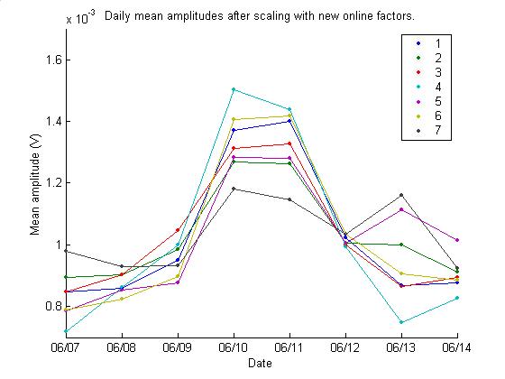
Online gain correction (scaling)
getMeanAmpOverTime
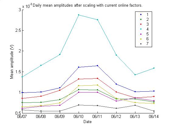
The online rescaling to correct for variation in gain from phone to phone appears to be broken. Perhaps this is because preamps were changed between February and June. Hopefully it can be fixed by calculating new scale values that are hard-coded in the online software. Below are given the mean amplitude of each channel, as determined by the 0.1 s samples captured every 10 minutes for 8 days from 6/7/02 to 6/14/02. Phone 4 is seen to be significantly higher in mean amplitude, indicating its gain has changed since the online scaling factors were last determined. This explains why phone 4 has recently been contributing 80% of the events.
Based on the mean amplitudes, new online scaling factors were determined. They are shown below along with the current factors. The factors are simply in the ratio of the mean amplitudes, normalized so their average is 1.
8/2/02
Jack’s data transfer
guidelines
A reminder, from Peter Camilli’s email to Giorgio 9/11/01:
100 kB can be transferred any time
1 MB can be transferred between 5pm and 7am, or during non-testing periods.
> 2 MB must be transferred by snail mail
So for transferring samples of data to check their validity, typically 5 minutes of data will be ~5 MB uncompressed and 1-2 MB zipped.
8/2/02
New online code
The online code has been updated by fixing the scaling factors, and Dan at Site 3 will install it.
8/2/02
Time zone confusion
2002.12.22 hour created is one hour later than name of file
2002.01.01 differ
2002.01.05 differ
2002.01.10 differ
2002.01.15 differ
2002.01.16 differ
2002.01.17 differ (at beginning)
2002.01.18 differ (at end)
2002.01.19 agree (at beginning)
2002.01.19 agree
2002.01.20 agree
2002.03.31 agree
So the hour springs back suddenly one hour.
Dan is checking on the time there – whether it’s Bahamas or California.
…Dan checked and says the PC is on Bahamas time, off by about 1 minute (email from Dan to Justin, 8/5/02)
8/2/02
Time differences
dtDistribution
I think Yue’s plot has no time differences between 0.1 s and 1 s because it is only those events captured for 10 ms. A plot of all events for one hour, as shown below, has no holes. Y`ue is also cutting on peak pressure > 0.5 Pa and a certain frequency range. He’ll plot all frequencies and all peak pressures for 10 ms events.
8/5/02
Event rates by phone
getEventRatesByPhone
Due to phone 4’s apparent higher gain, it triggers very often, contributing 75% of all triggers:
8/5/02
Coincidence diamond numbering
coincidenceDiamond
The diamonds are numbered as follows:
Diamond Phones
1 1 2 3 7
2 2 3 4 7
3 3 4 5 7
4 4 5 6 7
5 1 5 6 7
6 1 2 6 7
8/5/02
Coincidence depth profile
getEventDepthDistribution
hyperbolateLists on 2001.12.27.06
produces 6330 events in two branches (from the intersection algorithm), plus
and minus. Only those between depths 0
and 1600 m can be physical. 8% of the
plus solutions are in this range; 1% of the minus solutions are. None of the events in this set have both
plus and minus solutions with physical depth.
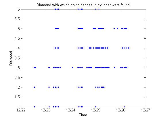
8/5/02
Rate of events in fiducial cylinder
getFractionInCyl
Further restricting reconstructed
events to lie in the horizontal circle circumscribing the outer phones does not
further restrict the number of events.
This is appears to be a good method for choosing between the plus and
minus solutions.
8/5/02
Events in multiple reconstructions
countUniqueEvents
Of 596 reconstructed events during
the hour 2002.12.27.06, we would ideally have 596 * 4 = 2384 unique
single-phone events that contributed to them.
However, the same single-phone event can be used in multiple
reconstructions. Single events are
actually being used in very many different reconstructions: instead of 2384
unique single-phone events, we have 91.
These could have come from at most 91/4 = 22 actual acoustic events, not
592. One single-phone event contributed
to 258 different reconstructions.
8/5/02
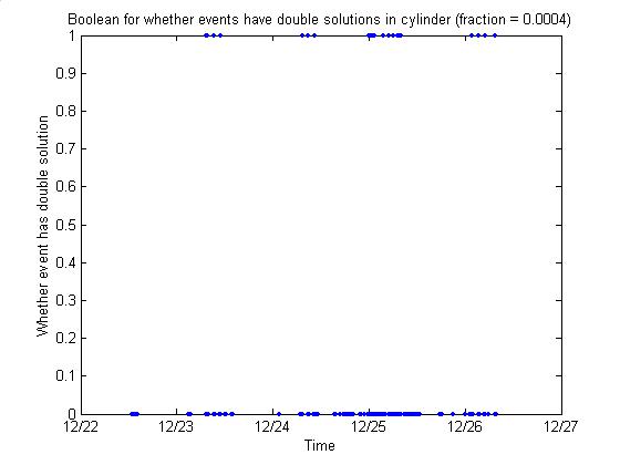
Events with two valid intersections
restrictToCyl
Two such events have been found, in
hyperbolateLists.2001.12.27.04. For
both events, the two intersections are within 50 m of one another.
8/5/02
Removal of events outside fiducial
cylinder
hyperbolateListsCyl
Files have been created with only
those events in the fiducial cylinder, reducing the number of events to 1/10 of
previous size:
hyperbolateLists…mat 147 files 9.0 MB
hyperbolateListsCyl…mat 147 files 0.9 MB
8/5/02
Time of day of coincidences
plotReconstructedTimes
For five days of continuous data,
coincidences were reconstructed, events outside the cylinder were rejected, and
histograms of time of day were produced.
The two peaks centered at 5am and 8pm that Yue found are perhaps
discernible, but it’s uncertain.

8/5/02
Maximum channel vs. triggering
channel
mChanVsTChan
The two differ 7% of the time.
I will switch from mchan to tchan
for most purposes.
8/6/02
Arrival time differences for
coincidence events
DtDistributionOfCoincidences
I checked the time differences
between single-phone events used to reconstruct acoustic events. The distribution is dominated by a delta
function at 0, because the same single-phone events are used so much. Then there is a much lower ~ Poisson
distribution.
8/6/02
Distribution of seconds of events
secondsDistribution
Because the online code performs
some tasks periodically with a period of one minute, there may be some
one-minute periodic deadtime resulting in an event rate with a one-minute
period. There does appear to be a small
effect:
8/6/02
Overflows
countOverflows
An overflow occurs when the event
rate is too high, so not all digitized samples can be processed, so some are
overwritten in their buffer. The
overflow rate is steady, as shown below.
The average rate is one every 4 minutes. ~20 s of samples are dropped by each overflow, yielding a
dead time of (20 s) / (4*60 s) = 8%.
8/7/02
Negative time differences
negativeDtRate
Occasionally, as events accumulate,
the time stamp of the event jumps backwards.
The rate of this occurring is shown below. The average rate is 6/hour.
Most of the negative time
differences are close to one value:
Same histogram with smaller bins:
8/7/02
Negative time difference related to
waveform length
negativeDtRate
In the online code, scans/waveform
is set to 20480. With a dt between
scans of 5.6 us, this corresponds to 0.11469 s. The longest negative time difference is 0.11468 s.
8/7/02
Negative time differences caused by
high event rate
negDtVsEventsPerMinute
There is positive correlation
between event rate and negative time differences:
8/7/02
ADC limits
The acquisition card’s ADC limits
are set to +/- 1 V, corresponding to +/- 7 Pa.
Is the ADC 16 bit? That is consistent with the 2 bytes/sample
given in the entry below.
8/7/02
Online scan buffer; limited by
memory
According to the LabVIEW context
help from pointing at the buffer size control on the SAUND.vi front panel, the
buffer size is memory limited. The size
is currently (3e6 scans) * (7 channels)
* (2 bytes) = 42 MB.
8/7/02
Number of events bug
checkNumEvents
compareNumEvts getNumEvts
For some time the number of events
per hour has not matched the sum of the number per minute. The number of events per minute is read
directly from a minute’s succeeding minutely data file in getNumEvts. Zero was
always returned for minutes of the form hh:59 because the minute incrementing
did not work. This has been fixed.
8/7/02
Coincidence candidate event rate
countCoincidenceEventLists
In one week of data from June 2002,
there are on average 30 single-phone coincidence candidates per hour, giving at
most 30/4 = 7 4-phone coincidence events per hour. Of ~200 time series seen in a couple hours of data, however, the
events are mostly noise. The number for
each hour are given below.
8/7/02
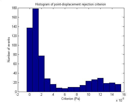
Single-point
displacements
findPointDisplacements
Many 10-50% of the single-phone
coincidence candidates are events that consist of single-point
displacements. A cut was developed to
reject these. The algorithm is as
follows: A list of the absolute value of the amplitudes of the pressures of the
event is made and sorted. For
single-point displacements, the greatest amplitude in this list is much greater
than the second-greatest. The rejection
criterion is thus the difference between the greatest and the next-greatest. A histogram of this number for the ~600
single-phone coincidence candidates during June 7-14, 2002 is shown below. The histogram shows two regimes, one on
either side of 6 mPa. Rejecting events
with a value above 6 mPa rejects most of the bad events and does not reject any
good ones, as determined by viewing the time series of all events of these ~600
above 6 mPa. Unfortunately computing
the criterion takes almost 1 s per event.
8/8/02
Point displacements in coincidence
candidates
removePDFromCEL
plotRemovePDFromCEL
27% of the single-phone coincidence
candidates in June 7-14, 2002 are point displacements.
When these are removed from the
coincidence event lists, most groups no longer form a complete diamond of hit
channels, meaning reconstruction of an acoustic event is rejected.
8/8/02
Negative time differences
timeProfile
Following is a profile of the event
rate for an hour in which many negative time differences occurred.
A close up of the same figure
follows. The horizontal lines on either
side are overflows.
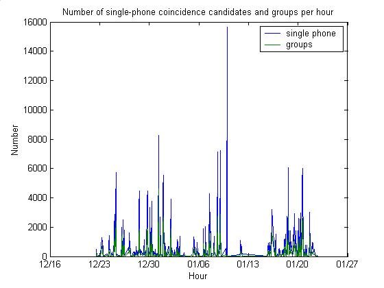
8/8/02
Coincidence in December-January vs.
June
countCoincidenceEventLists
There are many more candidates in
the Dec-Jan period than the June week.
Average rates:
June: 29 single-phone
events per hour 10 groups per hour
Dec-Jan: 593 single-phone
events per hour 313 groups per hour
8/8/02
Channel 4 dominance is not new.
8/9/02
Loud coincidence candidates.
plotLoudestCandidates
The loudest ~200 candidates from are
all diamonds. The loudest few hit the
rails at 7 Pa.
8/9/02
Loud groups of candidates
plotLoudestQuadsQuick
A coincidence event list consists of
multiple groups. A group is one
single-phone event along with all single-phone events following it that satisfy
timing and diamond criteria for a coincidence.
Rather than trying all possible combinations of events within a group
(there can be tens of thousands), I choose the loudest event at each
phone. The 4th loudest is then a
measure of the loudness of the loudest four.
Two categories of events follow,
tripolars and diamonds. An example of
each follows. Note that the events in
all channels are very loud.
8/14/02
Problem with MATLAB solved
I was using MATLAB 5, which suddenly
would not run (quit immediately upon running).
I removed it and installed MATLAB 6 (Release 12), but it similarly would
not run. After two days with tech
support, Jordan Schmidt at MathWorks realized it was because hep26 is a Pentium
4. P4 is not supported by MATLAB R12
but by R12.1. But there is a workaround
for R12 that I followed successfully (email to Justin from Jordan Schmidt,
8/14/02).
8/14/02
Better determination of new online
scale factors
getMeanAmpEvolution
I was unsatisfied with my online
scale factory calculation. I wanted to
see how much the mean amplitudes varied on a daily time scale. Below are the mean amplitudes of each
channel for three data ranges (Dec-Jan, Feb-Mar, Jun) with the current online
scale factors. The current online DC
values were removed before determining the mean amplitudes. Cross-talk was not removed.
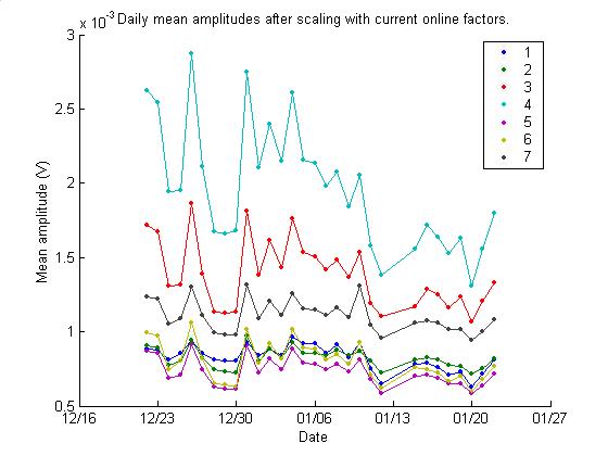
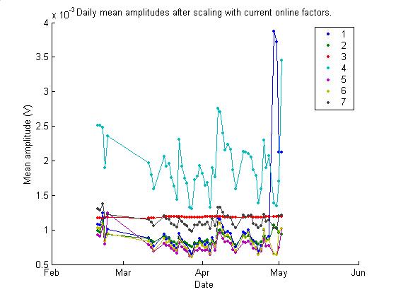
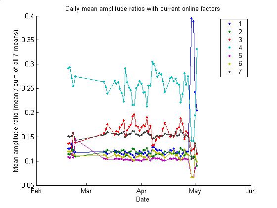
In the above plot, changes in the
amplifiers can be seen. Phone 3 is
disabled and terminated during the entire period. Phone 1 misbehaved in late May and then was terminated.
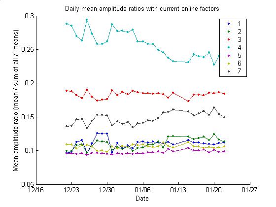
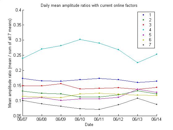
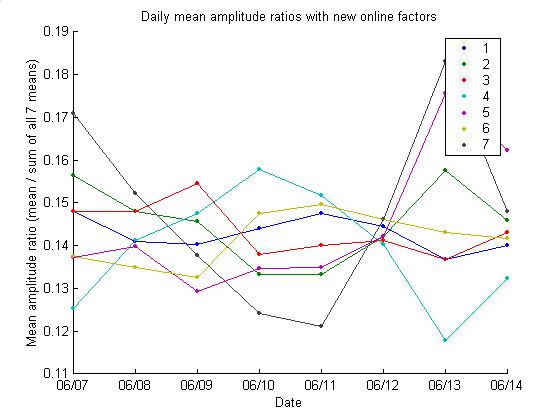
These plots include some coherent
variation in all 7 phones. Presumably
this is due to weather variation that covers the entire array. If the conditions vary similarly at all 7
phones, the ratios of the means should remain constant. The three plots below show the evolution of
these ratios (for each day, the ratios are the phone means divided by the sum
of all 7 phone means).
The new version of the code
calculates a new best scale value, which if it had been used in June would have
given the following two plots. Note
that the channel amplitudes are nicely randomized; their amplitudes listed by
phone are not always in the same order as in the above plot (with old scale
values).
The new best scale values, as
determined by getMeanAmpEvolution, are as
follows:
Only the week of June data currently
available have been used to determine these, as they are the only data
available since the amplifiers have been changed.
A new version of the online code has
been implemented with these factors, AUTEC_programs_2002.08.14.
8/14/02
Larger acquisition buffer
I added 512 MB (from 128 MB to 640
MB) of memory to hep26 to increase the acquisition buffer size. If all of this memory were used by the
acquisition buffer, it could increase in size by (512e6 bytes) / [(2 bytes/scan/channel)*(7
channels)] = 3.7e7 scans.
8/15/02
Merged event lists
mergeEventLists
It was confusing dealing with data
from some dates having eventList…mat files, and some having eventList2…mat
files, so they have been merged and now all have eventList…mat files.
8/15/02
Comprehensive event list
eventListComp
There was an error in the number of
events per hour in event lists, and I kept needing to add quantities. So there’s a new, comprehensive version of
event list that has been run on all data from June and Dec-Jan.
8/16/02
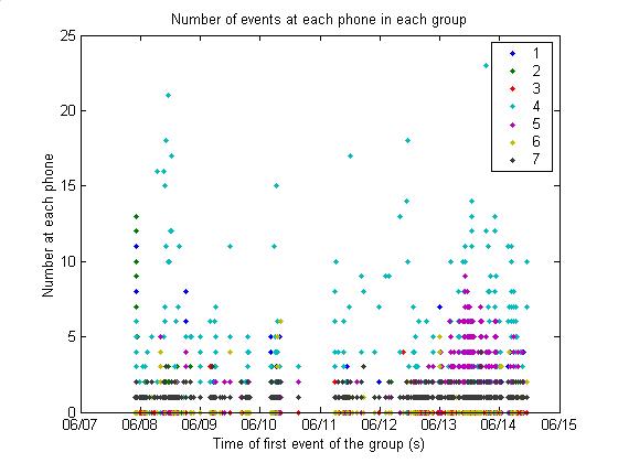
Number of events at each phone in
coincidence groups
CountGroupEventsAtEachPhone
plotGroupByPhone
Below is a plot of the number of
events in each coincidence group at each phone. This was run with coincidenceEventLists2, not
coincidenceEventListsComp. Note the
interesting higher rate of phone 5 on 6/13/02.
This gives a sense of the combinatorics problem: we have, typically,
fewer than 5 events at each phone in each group. At most one of these ~ 5 events must be chosen from each phone.
According to plotGroupByPhone, for this
data the phone of the first event of a group is never hit twice in one
group. This is what we want.
8/16/02
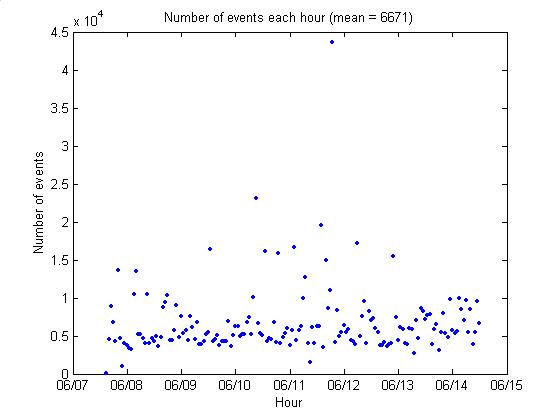
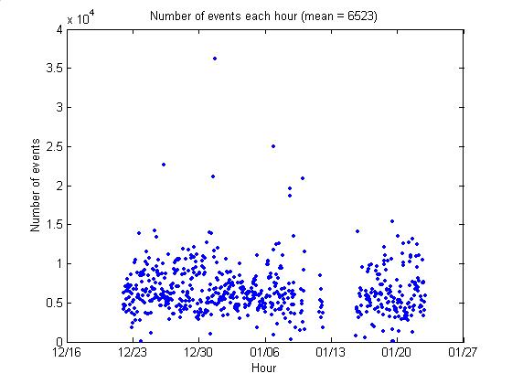
Number of events each hour
plotNumEvtsEachHour
Below are plots of the number of
events each hour for our two preliminary data ranges.
8/19/02
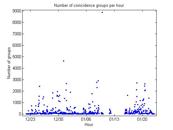
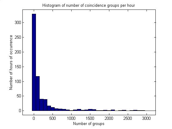
Number of coincidence groups per
hour
countGroupsPerHourOverTime
Below are a plot of the number of
coincidence groups per hour and a histogram of the number during the Dec 2001 –
Jan 2002 data range. The mean is
233. The standard deviation is 595.
8/19/02
Distribution of channels in groups
getChannelDistributionOfGroups
plotChannelDistributionOfGroups
In each coincidence group, each
phone is hit a certain number of times.
The phone of the first event should only be hit that first time (this is
not always true because of the negative time problem). On average, for the other 6 phones, when the
number of hits is sorted, there are 10 hits in the first, 4 in the second, 2 in
the third, and 1 in the fourth.
8/19/02
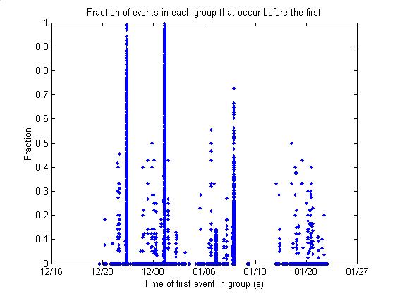
Fraction of events in each group
with bad timing
countCoincidenceNegDTs
PlotCountCoincidenceNegDTs
For each group, the fraction of
events with timestamp after the first event of the group was determined. A plot of this fraction vs. time of the
group is given below. Its average is
0.004, small enough to neglect the problem for most purposes.
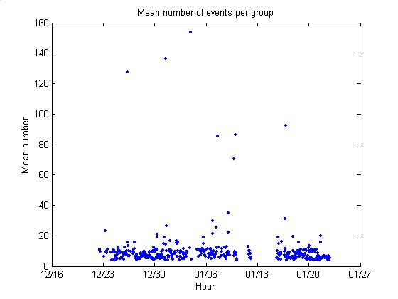
8/19/02
More coincidence group stats
countCoincidenceEventLists
8/20/02
Statistics from overnight
hyperboloid intersection run
readHyperbolateInCyl
hyperbolateInCyl
Below are plot summarizing the
results from searching for hyperboloid intersections that lie in the fiducial
cylinder over one night (ran for 12 hours).
It will take at least 80 hours to analyze all Dec-Jan data in this way. I beilieve the runtime is dominated by hours
in which a great number of events were captured in quick succession, resulting
in a very large number of combinations to check.
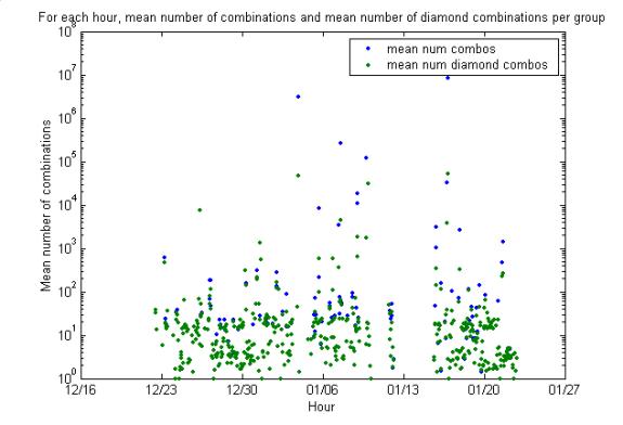
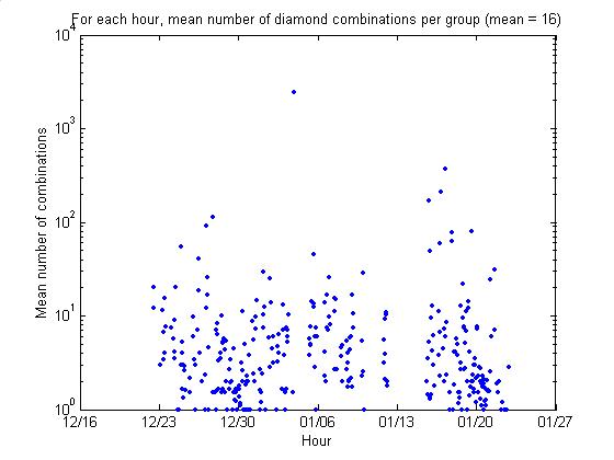
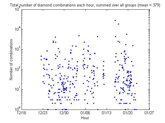
8/20/02
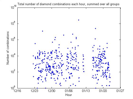
Rate of diamond combinations
countCombinations
plotCountCombinations
The first plot below is of the
hourly mean number of combinations per coincidence group, with and without
enforcing that the combinations form a diamond. They have means 7e5 (combos) and 2e3 (diamond combos) per
group. The second plot gives the total
number of diamond combinations for each hour, summed over all groups. The mean is 4e5. There are 3e8 total diamond combinations in the Dec 2001 – Jan
2002 dataset.
8/20/02
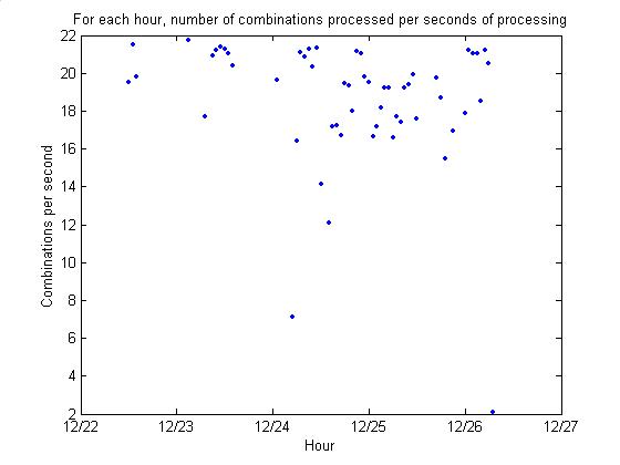
Hyperbola intersections search time
scales with number of combinations
readHyperbolateInCyl
The plot below gives the number of
diamond combinations processed per second during an overnight run of hyperbolateInCyl on
hep26. The mean processing rate is 19
combinations per second. For the Dec
2001 – Jan 2002 dataset, we have 3e8 total diamond combinations (see above), so
processing it all at this rate would take 4000 processor hours. However, by only processing those hours with
1e4 combinations or fewer, it is possible to analyze 369 of the 619 hours with
data in the Dec 2001 – Jan 2002 dataset in ~8 hours (see plotCountCombinations for this
calculation). This cut will analyze a
total of 5e5 combinations.
8/21/02
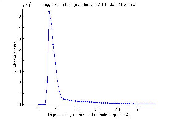
Histogram of trigger values
plotTriggerValHistograms
The plot below gives a histogram of
all trigger values for all events in the Dec 2001 – Jan 2002 data range. The events are fairly strongly clustered near
10 threshold step units, but there is a long tail that extends as far as 862
threshold step units.
8/21/02
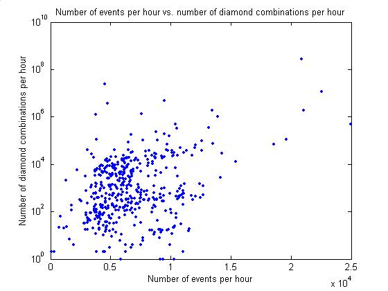
Poor correlation between event rate
and coincidence rate
plotNumCombinationsVsEvents
The plot below gives the number of
events per hour vs. the number of coincidence events per hour for Dec 22 2001 –
Jan 2002 data. The correlation is not
good. Presumably this is because we have
averaged over too long a period – an hour.
Perhaps events per minute vs. coincidences per minute would give better
correlation.
8/22/02
Negative time differences due to
reading the same 20480-scan buffer twice
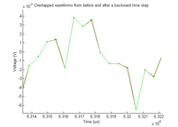
plotDoubleTimes
The same buffer of waveforms is
analyzed twice after a buffer overflow, resulting in events with the same
samples, as shown below.
It is still mysterious why the read
buffer is read twice immediately after an overflow. [Check if dead time is
16.800 s or 16.685 s]
It is also mysterious why the exact
same events aren’t captured, if the threshold is the same. [Check that
threshold is the same]
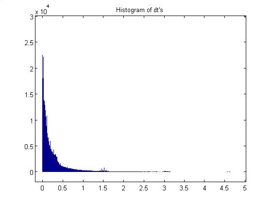
8/22/02
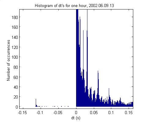
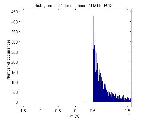
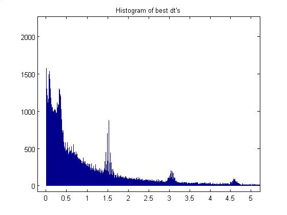
High-resolution dt histogram
dtDistribution
Below is the low-dt part of a
histogram of time differences between events for one hour of data. The second plot is two orders of magnitude
higher resolution. The hour has very
many overflows. The spike in the first
plot at –0.12 s corresponds to re-reading the read buffer of 20480 scans
spanning 0.12s, and jumping back to the beginning of that buffer. The 0.5 ms cutoff shown in the second plot
cutoff is that which prevents two events from capturing overlapping waveforms
(It should be 1 ms but is at 0.5 ms due to an online bug). We see that the threshold is much too low
and our trigger rate is limited almost only by the enforced 0.5 ms dt. This also explains why, even though the same
buffer is processed twice, we don’t trigger on the same events again – we
trigger mostly on those that are 0.5 ms after the previous event.
11/22/02
Rate of small dt’s
countSmallDT
Indeed, the bad hour shown above has
a very high rate of dt’s between 0 and 0.5 ms.
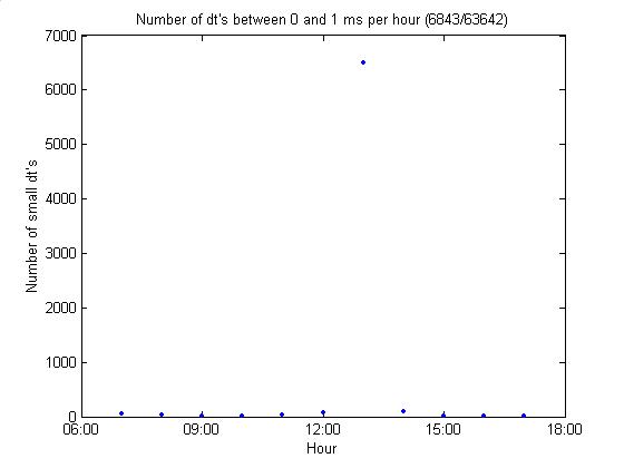
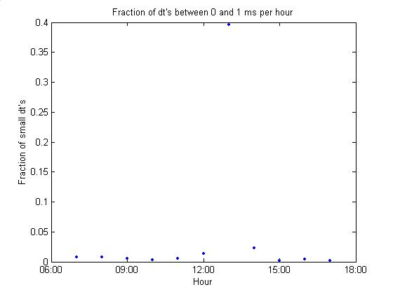
Below are the same two plots for two
ranges of hours.
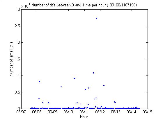
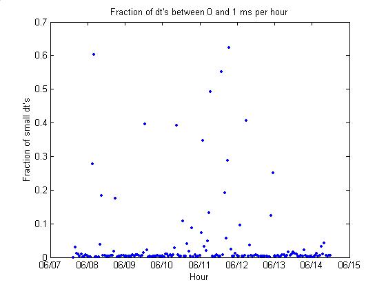
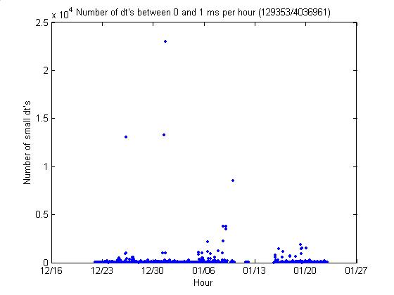
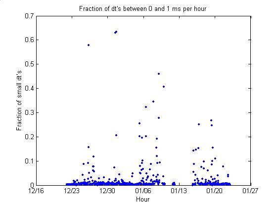
We see that up to 1/10 of all dt’s
are between 0 and 1 ms. Presumably these are what make coincidence
combinatorics so difficult.
8/22/02
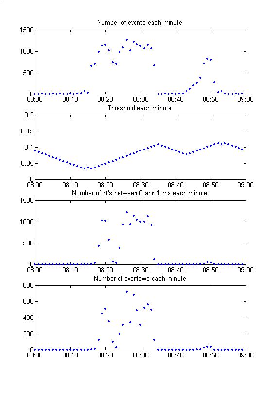
Poor threshold algorithm causes
triggering on rms noise
plotNumEvtsPerMinute1Hour
Below is a plot showing shows that
our poor thresholding algorithm results in increasing the threshold too slowly
in periods of high rms noise, which results in too great an event rate, which
results in overflows. Data are given
for one hour, 8am on 12/26/01, during which very many (13,000) small dt’s
occurred and the event rate jumped far over the target of 60/minute. A new adaptive threshold will quickly
calculate the new threshold it should jump to, rather than inching up to it
step by step.
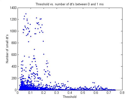
8/22/02
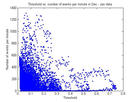
Very low thresholds guarantee an
event rate too high
plotThresholdVsNumEvents
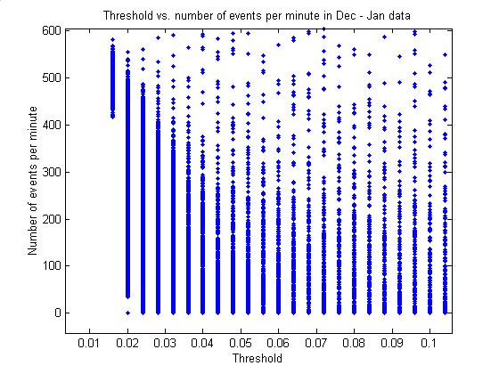
Below are a plot of threshold vs.
number of events for each minute of Dec 22 2001 – Jan 2002 data (first figure)
and close-up (second figure).
Thresholds only occur at discrete values. Note low thresholds guarantee a high number of events. This is the rms noise floor. In particular, a threshold of 0.016
guarantees an event rate of 400 events per minute or greater.
8/22/02
Low threshold does not directly
cause high event rate
plotThresholdVsNumSmallDTs
Threshold vs. number of small dt’s
per minute (ie threshold vs. rate of triggering on rms noise) does not show a
similar pattern. That is, triggering on
rms noise is not caused absolutely by having a low threshold, but by having a
low threshold relative to the current rms noise level.
8/23/02
Event codes
countEventCodes
All level 2 triggers are
written. Every 100th level 1
trigger is also written, whether or not it triggered level 2.
Each event is written with one of
the following identifying codes:
(0)
This event triggered both level 1 and level 2
(1)
A 100th level 1 trigger; also triggered level 2
(2)
A 100th level 1 trigger; did not trigger level 2
So to use all events that triggered
both level 1 and 2, use all events of both codes 0 and 1.
Below is a plot of the number of
events of each code per hour over time for the Dec-Jan data range:
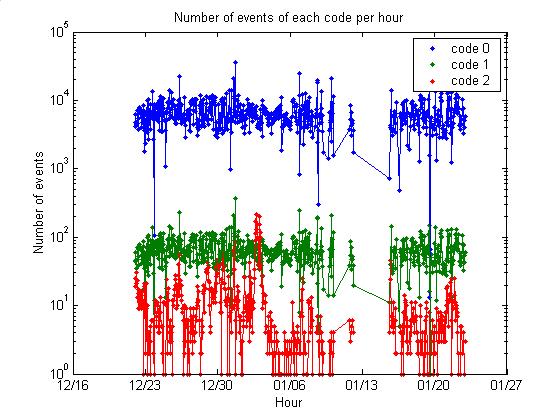
Code 2 events correspond to signals
highly correlated among all 7 channels (electric noise). Note that the rate is fairly variable over
time.
The mean rates of codes 0, 1, and 2
respectively are 6446, 65, and 11 events per hour. So the level 2 trigger rejection rate is 11/(11+65) = 14%. The percentage of events on disk that did
not trigger level 2 is 11/(11+65+6446) = 0.2%.
The rate of trigger 1’s written regardless of trigger 2 is 1.2%,
slightly higher than the ended 1% due to a small bug in counting trigger 1’s
online.
8/23/02
Event code 2 (correlated electric
noise)
plotCode2Events
Plotting time series of events with
code 2 verifies that they are corrrelated electric noise.
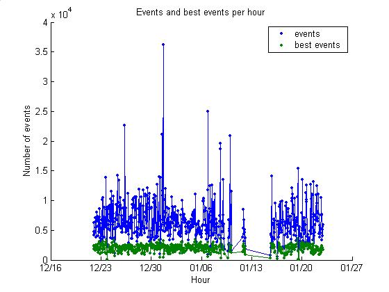
8/23/02
Removing all but ~ 60 events each
minute
keepBest60
plotKeepBest60
A second pass of thresholding was
attempted off line. For each minute a
threshold was chosen, restricted to integer multiples of 0.004, that would cut
all but as close to 60 events per minute as possible. The resulting event rates are given below. The means are 6523 and 2009 events per hour
(109 and 33 events per minute).
8/23/02
Effect of post-thresholding on dt
distribution
bestEventDTs
The plots below give the
distribution of time differences between events before and after offline
rethresholding. With rethresholding we
are les dramatically up against the noise floor. There are 1/10 as many dt’s at the low end of the spectrum. Dt’s are in s.
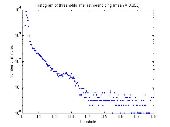
8/23/02
Effect of offline rethresholding on
threshold evolution
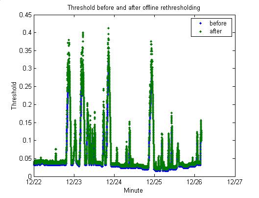
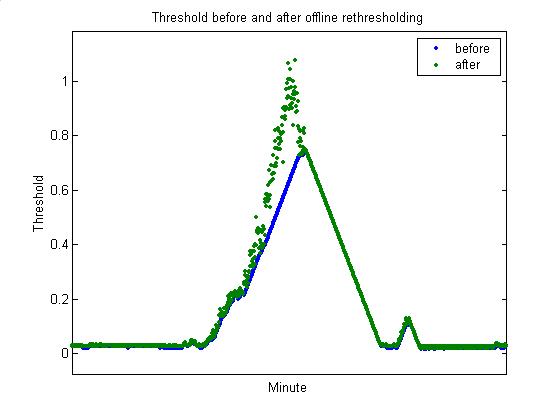
bestEventThresh
The plots below show the threshold
over time, before and after rethresholding (the second plot is a closeup of a
particular peak). The thresholds are
generally the same, differing primarily at the peaks of rapid ascents.
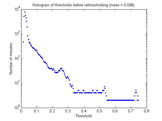
The plots below show histograms of
the threshold before and after offline rethresholding.
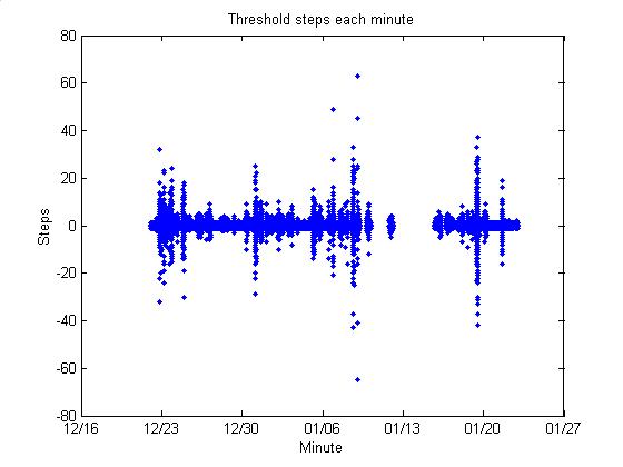
The plot below shows, for each
minute, the number of threshold steps that were taken to adjust the
threshold. Up to 60 steps are
taken. The current algorithm is limited
to +/- 1 step per minute.
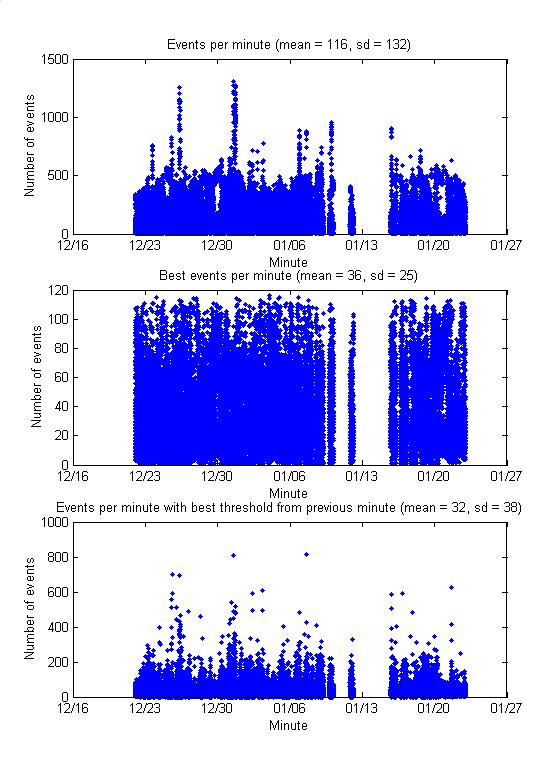
8/23/02
Events per minute
thresholdPrevMin
plotBestEventsPerMinute
The plots below show events per minute
before and after offline rethresholding.
Rethresholding effectively cuts down the event count of busy
minutes. The maximum changes from ~1300
to ~120 events per minute if the ideal threshold is determined for a minute and
applied directly to that minute (2nd plot). The 3rd plot shows calculating
the ideal threshold for a minute and then applying it to the following minute,
as would happen online. It is not
nearly as stable as applying the threshold directly to the same minute (2nd
plot), but is better than the current algorithm (1st plot). Perhaps we could hold an entire minute of
data in memory online and read through the data once to determine the threshold
before selecting events and writing them to disk. The title of each plot gives the mean and standard deviation.
8/26/02
Coincidince combinatorics with
offline rethresholding
bestCEL
countCombinations
plotCountCombinations
Coincidence groups were determined
from only the events that passed offline rethresholding (a small fraction of
events with code 2 were simultaneously removed). Those that no longer formed diamonds were removed. Below are the resulting statistics. In the Dec – Jan data range, there are now a
total of 1.2e5 combinations (cf 3e8 previously). At a processing rate of 19 coincidences/second, it will take ~ 2
hours to calculate hyperboloid intersections for all combinations (cf 180 days
previously!).
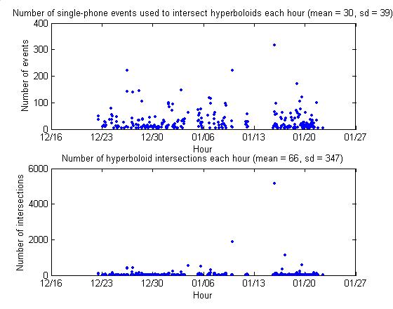
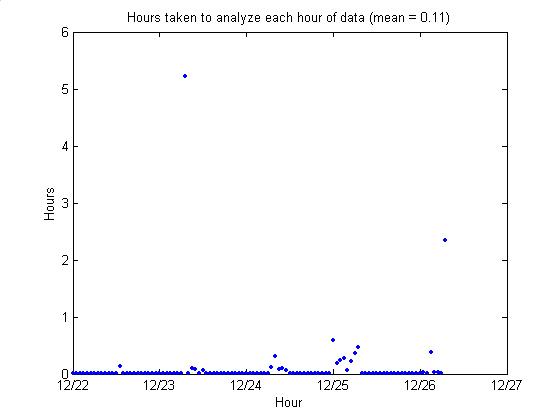
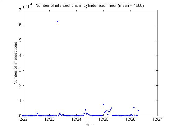
8/26/02
Intersection statistics
countIntersections
The second plot below gives the
number of hyperboloid intersections found each hour. The first plot gives the number of single-phone events used to
construct the intersections. When there
is no redundancy (when no single-phone event is used in multiple
intersections), we expect the quantity in the first plot to be 4 times the
number in the second, however it is ~1/2.
So we still must reject 7/8 of the intersections.