Log 2

Justin Vandenbroucke

justinv@hep.stanford.edu

Stanford University

8/26/02 – 9/24/02

This file contains log entries summarizing the results of various small subprojects of the AUTEC study. Each entry begins with a date, a title, and the names of any relevant programs (Labview .vi files or Matlab .m files – if an extension is not given, they are assumed to be .m files).

8/26/02

Event energy spectrum

eventSpectrum

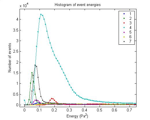
Below is a plot of the energy spectrum of events. Event energy is defined to be the sum of the pressure (in Pa) squared over 179 samples. The DC offset is removed before squaring. RMS noise is not removed. In the dominant channel (4), there appears to be an exponential spectrum in addition to some small peak between 0.2 and 0.3 Pa². All events from Dec 01 – Jan 02 are plotted.

8/27/02

Negative time differences – LabVIEW problem

SAUND test double buffer read.vi

check times.vi

I confirmed that LabVIEW reads the same sequence of 20,480 samples twice in a row following an acquisition buffer overflow. Spencer at NI is checking on this problem and on why I can’t use the extra 512 MB of memory added to the machine.

8/27/02

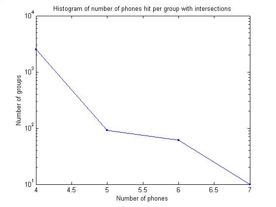
Search for coincidence with more than 4 phones

phonesPerGroup

Below are two plots showing the number of phones hit per group (counting only groups with intersections in the fiducial cylinder). In the Dec – Jan data, there are 10 groups with 7 phones hit. Plotting time series shows events that are loud, above the noise, and with similar shapes.

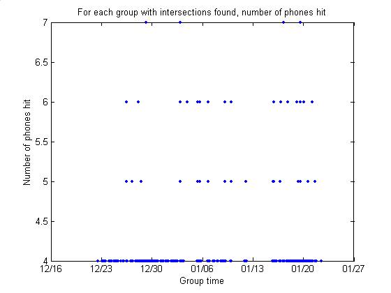
Combinatorics is still a problem for 7-phone events. Several of these groups are composed of 28 events, with only one of 7 events.

8/28/02

ADC numbers

From C:\AUTEC_analysis\text files_2002.08.07\NI documents \card.pdf (PCI E Series User Manual), the possible ADC ranges are +/- 0.05, 0.01, 0.25, 0.5, 1, 2.5, 5, 10 V. The range is currently set to +/- 0.5 V, giving a pressure range of +/- 7 Pa. According to Nikolai’s paper, the expected amplitude for a hadronic shower of energy 10²⁰ eV at 1 km is 0.4 Pa (0.08 Pa for EM shower) , so this should be sufficient. The card (National Instruments PCI-MIO-16E-1) has a 12-bit ADC, 1 sign bit and 11 magnitude bits. So with a range of –0.5 to +0.5 V, the least significant bit and ADC precision is 0.5/2¹¹ = 0.24414 mV = 3.4486 mPa.

8/28/02

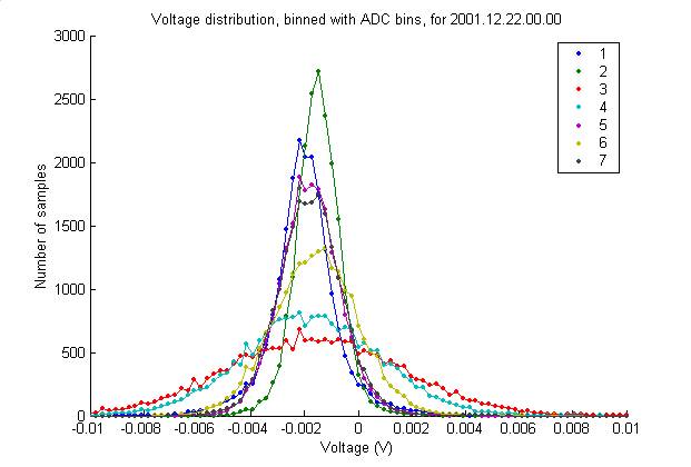
Gaussian noise

calcNoiseDistribution

plotNoiseDistribution

We never checked the gaussianity of the white noise. Below is a histogram of 20,480 consecutive voltage measurements (spanning 0.1 s). The bins are exactly the possible output values of the ADC. The DC offset is clearly visible, as is the variation in phone noise levels. Presumably the variation is in the hydrophone gains and not the noise environments of the phones.

8/28/02

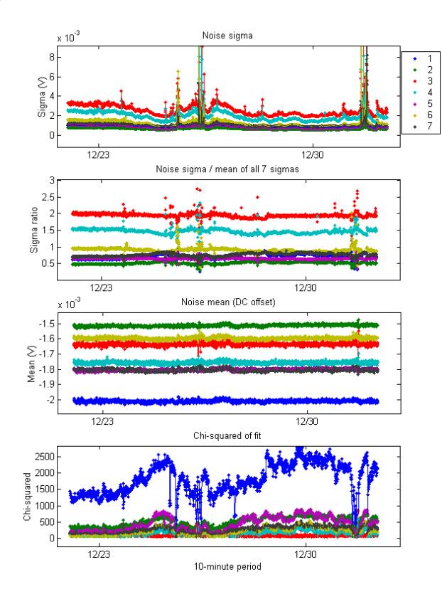
Fits of gaussian noise

fitNoiseDistributions

plotNoiseFits

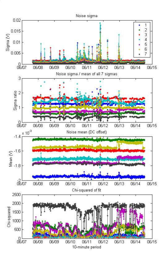
For each 10-minutely 20,480-sample, 0.1 s waveform, a gaussian was fit to the voltage distribution of each phone. Below are the results for 250 hours in Dec – Jan (first plot) and 166 hours in June 2002 (second plot). These should be better determinations of noise level and offset than previous ones. Note in the second plot that the DC levels of two channels change abruptly for a day and a half and then return to their previous values.

8/28/02

Noise variation with time of day

plotNoiseVsTimeOfDay

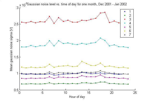
Below is a plot of gaussian noise sigma vs. time of day for one month of data. There is perhaps a slight change at dawn and dusk, but it is not a significant difference.

8/29/02

Online code improvements

Solved the negative dt problem in the online code: see AUTEC_programs_2002.08.29\version_history.txt.

9/4/02

Samples above threshold per event

triggersPerEvent

plotTriggersPerEvent
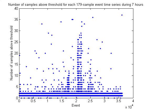
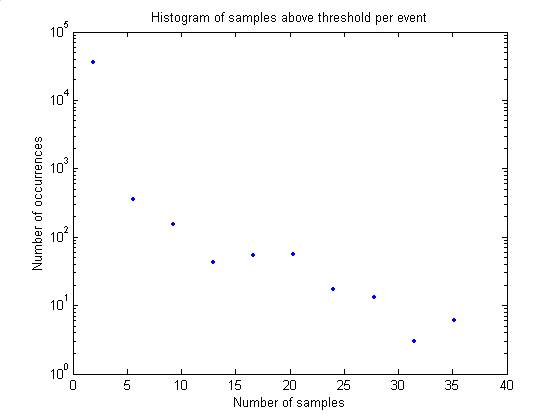
A difficulty with the histogram method of thresholding is that there are multiple samples of the filtered signal above threshold in each 179-sample event capture. In the histogram, should we count each sample or enforce a separation of 179 samples? Below are data on the number of samples above threshold per event for 7 hours of data.

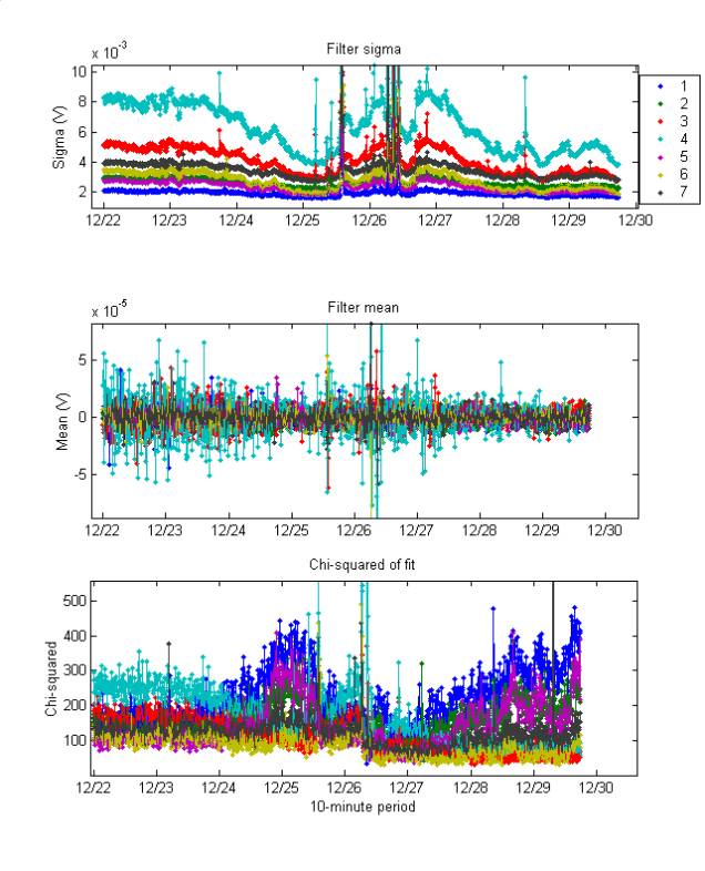
9/4/02

plotFilterFits

Filter gaussian fits

The filtered signal is dominated by Gaussian noise, as it should be (filtering a gaussian signal results in a gaussian signal). Below are data on the evolution of the fits to the gaussian distribution of filter values, taken every 10 minutes. Recall the threshold mean is 0.024, with a range from 0.016 to 0.104.

9/4/02

Overall noise distribution

fitOverallNoiseDistribution

The plot below gives histograms for the gaussian noise including all 0.1 s samples taken every 10 minutes for 120 hours. The 120 hours have a stable DC offset (two channels jump DC values for ~40 hours succeeding these and then jump back to their previous values).

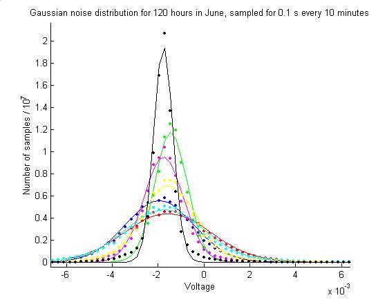
The table below gives the fit parameters for the gaussian distributions. These values will be used as the best value for online DC removal and gain rescaling. Online DC is the current hard-coded value removed online before analysis. Best scale factors are simple sigma / mean of all 7 sigmas.

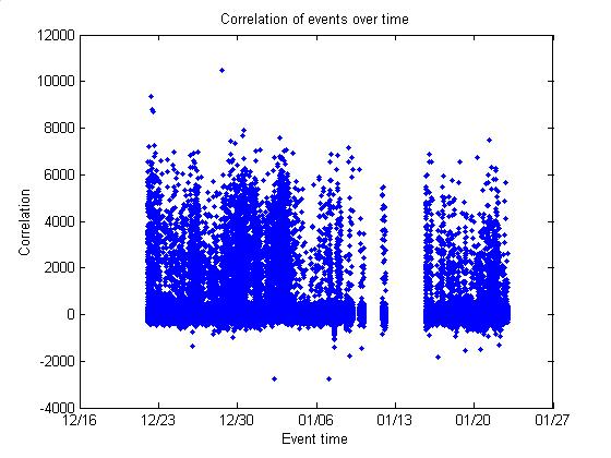
9/5/02

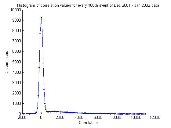
Correlation

checkCorrelation

Below are data for the correlation of every 100^th trigger 1 (which is written independent of trigger 2). Currently, trigger 2 requires that the correlation is less than 500. Its rejection rate is 15%. 4/1000 of the events have correlation less than –500.

9/11/02

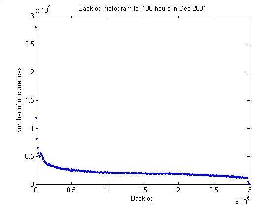
Dependence of overflow rate on buffer size

plotBacklog

The plot below gives a histogram of the backlog (measured every time an event occurs). Overflow occurs at 3e6. Also, by counting the number of times the overflow goes above a number, the hypothetical number of overflows that would result from a buffer of that size can be determined. For 1e6 samples, we would have an additional ~15 overflows / hour, twice the current rate. This is without taking into account the good effects of the improved thresholding algorithm, which should lower the overflow rate.

9/16/02

Regular point displacements

plotPointDisplacements

Point displacements were determined by requiring that the difference in amplitudes between the two largest-amplitude samples, divided by the largest amplitude, is above 0.7. Below is a histogram of this rejection criterion.

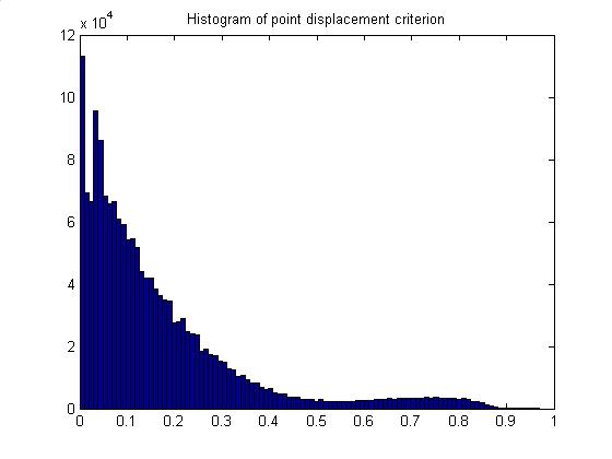
Time differences were determined between these point displacements. These events largely explain the 1.5 s periodic structure, as shown in the plot below.

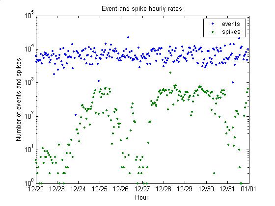
The plot below shows the rates of all events and of point displacements. The overall rate of spikes (point displacements) is 3 %.

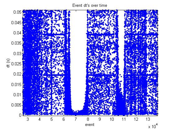
9/16/02

Periodic structure in all events

dtDistribution

The plots below show consecutive event dt’s for all events.

In the first plot below, structure every 20 ms is evident (50 Hz). 60 Hz would be every 0.01666 s.

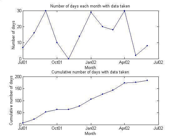
9/19/02

Summary of data taking in the past year

daysOfData

We have taken data for over a year now. It would be interesting to do some analysis of noise levels over the course of the entire year. To do this we would ideally have some data taken every day. Below are two plots summarizing during which days any data were taken. Since we began running, about half of the days have some data. The plots are complete up to the last shipment of data, which contained through mid – June 2002.

9/19/02

Gaussian noise over time

plotMinutelyNoiseEnergies

Noise power spectra are written minutely. In each spectrum, 512 values are written for each channel. Each value gives the power at a particular frequency, in steps of df = 1/512/(5.6e-6 s) = 349 Hz. The first value gives the DC power, which is very high due to the DC offset. Indexing from 1 (which is the DC power), the ith value gives the power at frequency df * (i-1). The 257^th value gives the power at the Nyquist frequency, 256*df = 89 kHz (half of the sampling frequency). The 255 values following the Nyquist frequency are redundant: Y_257+i = Y_257-i for i from 1 to 255, where Y_j (j from 1 to 512) are the power values. The first half represents positive harmonics, while the second half represents negative harmonics. The power of the jth harmonic (j from 2 to 256) is Y_j + Y_514-j = 2Y_j. The DC and Nyquist powers are Y₁ and Y₂₅₇, respectively. So the total non-DC power is the sum of all elements of Y from 2 to 512.

Minutely spectra are calculated from the first 34*512*5.6e6 s @ 0.1 s of data. They are determined by using the LabVIEW standard function Power Spectrum on 34 consecutive time series of 512 samples each. These 34 power spectra are then averaged. Online, the values are then divided by df (to convert from power to power per unit frequency) and multiplied by 2 (so that the harmonic powers are given by Y_j rather than 2Y_j). Nikolai implemented these two conversions but I find the default easier to work with so I reverse them offline (multiply by df and divide by 2). The minutely noise energy is then defined as NE = v2p * v2p * 179 * sum(spec(2:end,:)) * df / 2, where spec is the power spectrum on disk and v2p is the conversion factor from Volts to Pascals. This value is now equivalent to the sum of 179 Pressure values squared. It is therefore suitable for direct comparison to event energies. The noise values are not rescaled by the individual phone gains.

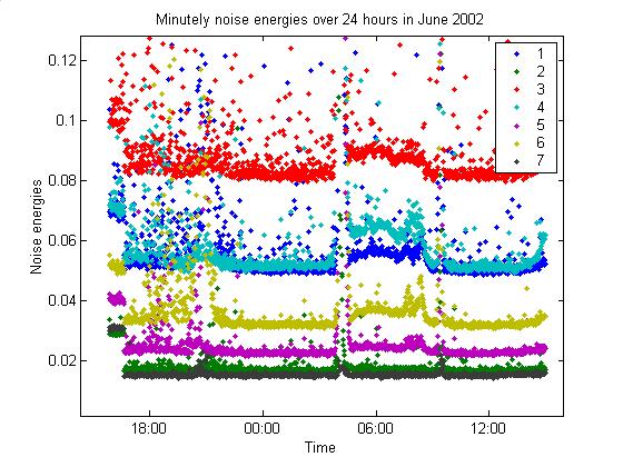
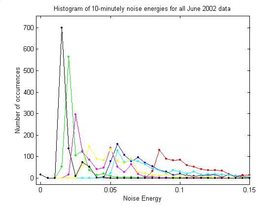
The plots below give noise data for all data available in June 2002.

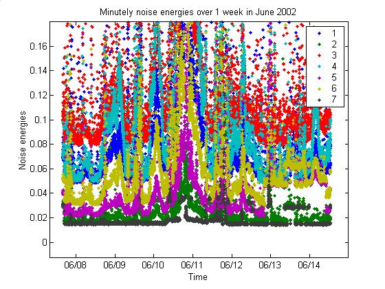
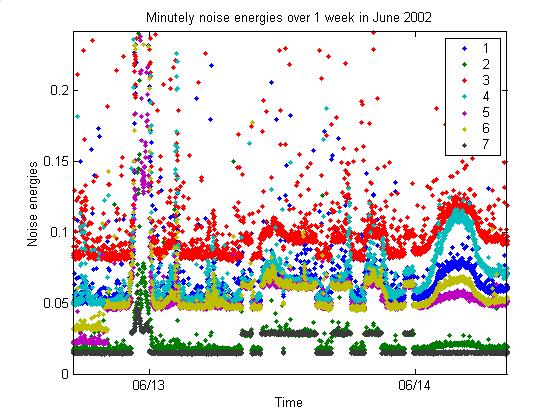
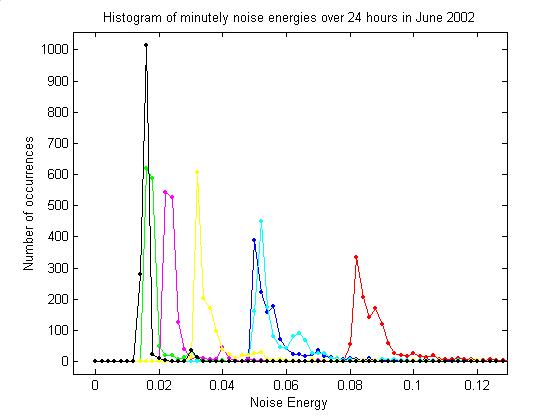
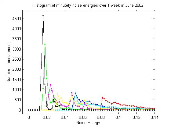
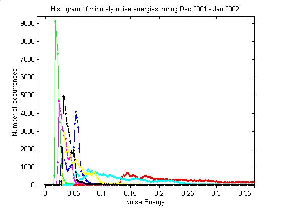
The first plot below shows a close-up of the noise during a couple days. Note that the noise level in all 7 channels strangely jumps back and forth several times between two discrete values. The second plot shows a histogram of noise energies for Dec 2001 – Jan 2002.

The first plot below gives, for comparison, a histogram of event energies. All events from Dec 01 – Jan 02 arge plotted. See the 8/26/02 log entry for details. The second plot

9/20/02

10-minutely time series noise

plotNoiseEnergies

Every 10 minutes a 0.1 s time series is written. With DC removed, 179 * <P²>, where P is the pressure, of this series should give a measure of the noise that is equivalent to the minutely calculation shown above from the power spectrum (it is also directly comparable to event energies). Compare the plot below to that above for all June 2002 data.

9/20/02

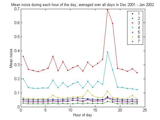
Noise variation with time of day

plotNoiseVsTimeOfDayMinutely

The plot below gives the mean noise in each channel for each hour of the day, averaged over about one month of data. There appears to be a significant spike in all channels at dusk.

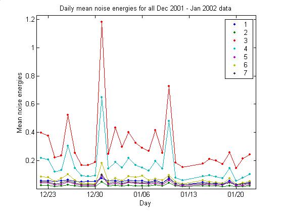
9/20/02

Daily mean noise energies

plotDailyNoise

The plot below shows daily mean noise energies for each channel. There are a couple exceptionally noisy data, but this is too short a period (1 month) to see seasonal variation.

9/20/02

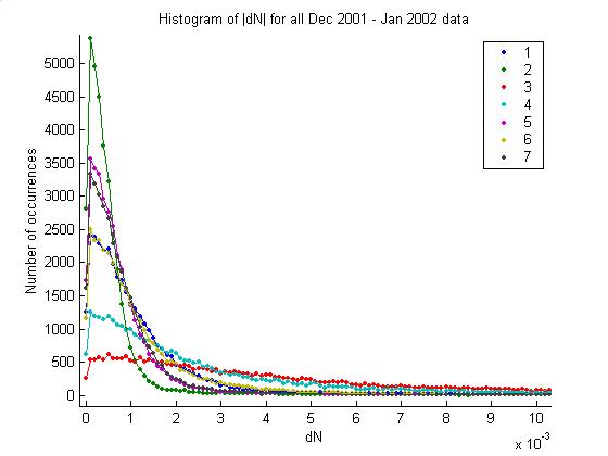
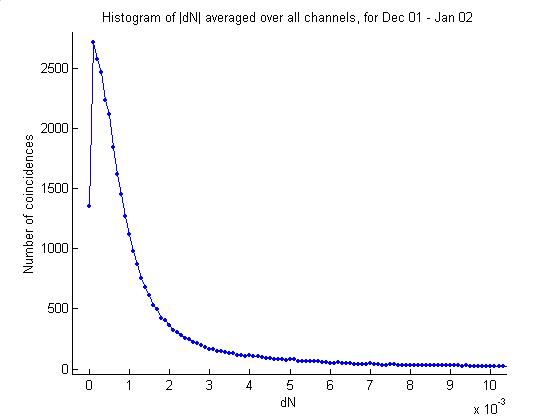
Noise volatility

noiseVolatility

Unfortunately the noise energy varies a great deal over short time periods. The first plot below is a histogram of |dN|, the absolute value of the difference in noise energy between two consecutive minutes. The distributions are peaked at small values but have very long tails. Note the variation in channels. Channel three is more volatile than the others. The second plot gives the average of the distributions over all channels. One-half of the minutes have mean dN (over channels) below 1e-3.

The table below gives the average value of |dN|, along with the average value of N (noise energy), for each channel (also for Dec 2001 – Jan 2002 data). Typically the noise energy varies by 1/10 of its value from minute to minute.

9/20/02

New online code

checkDanSampleMinuteData

Dan Belasco at Site 3 has installed AUTEC_programs_2002.09.15, and sent several minutes of data for me to check. There are a couple problems. The first is fairly small: the new direct thresholding from the previous minute’s distribution of filter values includes all filter values that are high due to electronic correlated noise. However, only 15% of level 1 triggers are rejected by level 2. So ideally our target event rate would be 60 / .85 = 71 events per minute. However, the rejection rate of 15% is fairly volatile and varies between 10 % and 90 %. 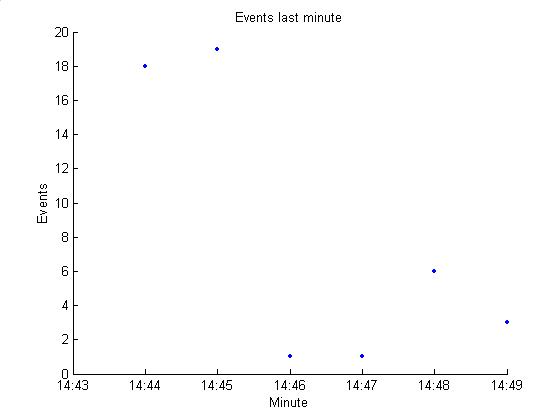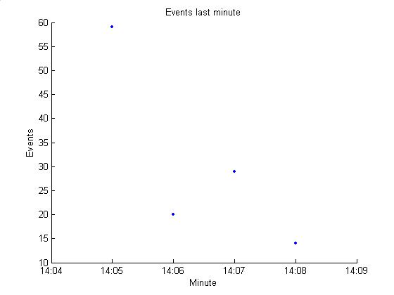In the sample Dan sent, there was an average of 10 events per minute (see plot below). Hopefully this is lower than typical and the average will be roughly 60 * 0.85 = 51 events / minute.

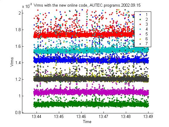
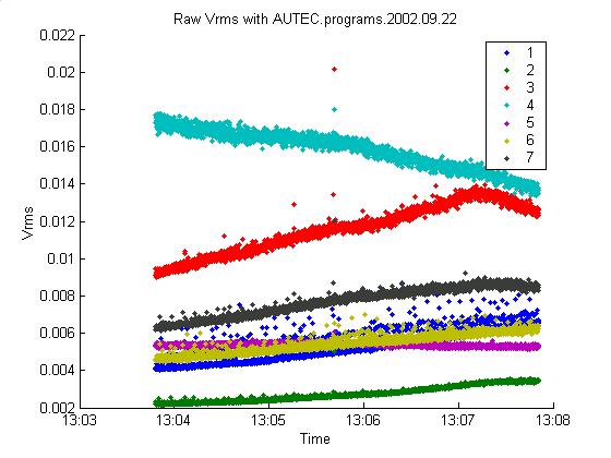
The new version writes Vrms every 0.1 s (in previous versions we could only calculate Vrms, or noise energy, once per minute – from the power spectrum). This will help analyze the volatility of the noise energy. Vrms for the sample Dan sent is shown in the first plot below. Unfortunately the gains appear to have changed again. The gain of channel 7 appears to have increased significantly while the other channels remained unchanged. Compare to the second plot below, pasted from a 9/19/02 log entry. Indeed, every single event (51 of them) in the sample Dan sent occurred at channel 7. Apparently we need to have automatic gain correction built into the program.

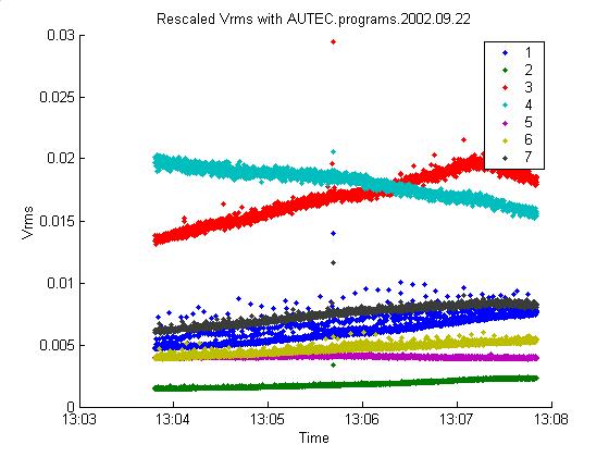
New scale factors can be calculated from these data. They are given in the table below. The new scale factors are <Vrms> divided by the mean of <Vrms> over all channels.

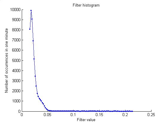
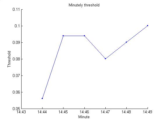
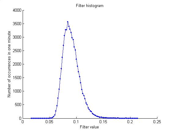
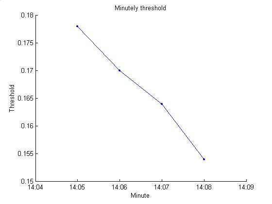
The new threshold algorithm is generally working well. Online, the stream of samples is filtered and then broken into 179-sample waveforms. The maximum of each waveform, if it is above 0.016, is added to a filter histogram. This is then used for the next minute to predict a threshold that will yield close to 60 events. The histogram is written each minute. The first plot below is an example. The second plot gives the threshold values. Previously the threshold could only change by 0.004 in either direction; now it can jump to any multiple of 0.002.

9/22/02

New online code

I sent a new version to Dan with the new scale factors. Also changed Vrms from rescaled to raw values. For some reason the first event of Dan’s sample had a zero-length time series (likely because of a failed call to get subarray), but I couldn’t reproduce the error or figure out why it would have happened.

9/23/02

Gain problems in channel 7

Dan emailed saying that there was a postamp problem with phone 7 that he noticed in July and fixed August 15.

8/23/02

AUTEC_programs_2002.09.23

Dan sent a sample of 4 minutes with the new data. They are summarized in the plots below. Note the very high Vrms values (typical values are 1 mV, while these are 10 mV). Channels 3 and 4 cross over. It looks like there may be a noise object (ship) moving through the array. The filter values are correspondingly much higher than usual (typical threshold is 0.04). The new scale factors appear to not be great. All 122 events occurred in channel 4.

9/24/02

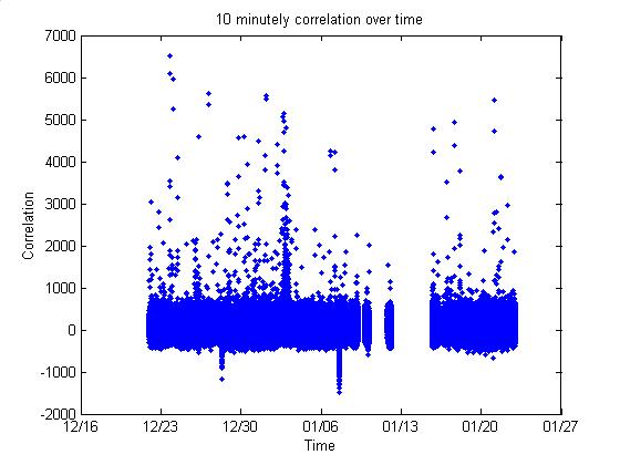
Correlated noise

plotTenMinutelyCorrelation

If spike noise occurs with a semiregular period, perhaps correlated noise does too. Indeed, it does. The plots below are all for the entire Dec 2001 – Jan 2002 data range. The 0.1 s time series written every 10 minutes were used to measure the correlation over time (regardless of triggering). Each 0.1 s time series was broken into ~100 subwaveforms of length 179 (1 ms). The same algorithm used to calculate the correlation in the online level two trigger was applied to each of these 179-sample waveforms. The first plot below shows all of these correlation values over time. 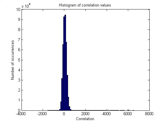The second plot gives their distribution. It is roughly gaussian near zero, with a negative tail and a longer positive tail (corresponding to correlated noise). 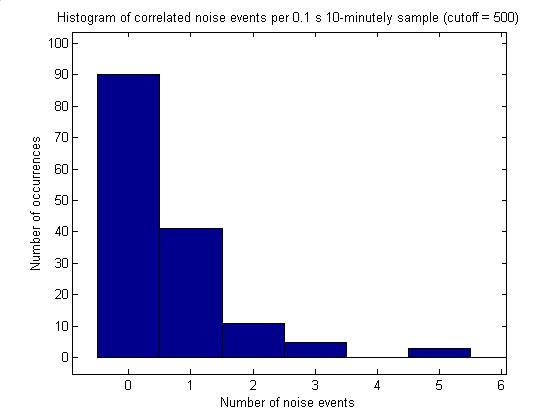The gaussian is centered slightly right of zero, likely due to residual cross talk (although most of the cross talk is removed ). As in the level 2 trigger, time series with correlation above 500 are considered to be correlated noise events. 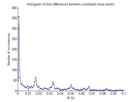A histogram of the number of these events per 0.1 s time series is plotted in the next plot. The final plot gives a histogram of time differences between correlated noise occurrences. The spike at 0.l ms is for when consecutive 179-sample subwaveforms are both correlated (the period of correlation stretches beyond 0.1 s). There are also spikes at multiples of 0.017 ~ 1/60 s, corresponding to a 60 Hz rep rate.