Log
4
Justin
Vandenbroucke
justinv@hep.stanford.edu
Stanford
University
10/17/02 – 11/1/02
This file contains log entries summarizing the results of various small subprojects of the AUTEC study. Each entry begins with a date, a title, and the names of any relevant programs (Labview .vi files or Matlab .m files – if an extension is not given, they are assumed to be .m files).
10/17/02
Event correlations
eventCorrelations.m
calcCorrelationDistribution.m
plotCorrelationDistribution.m
removeXTalk.m
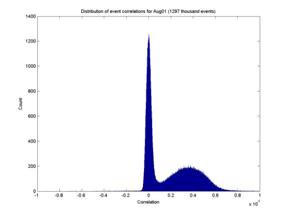
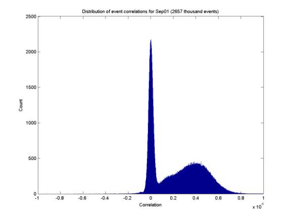
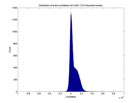
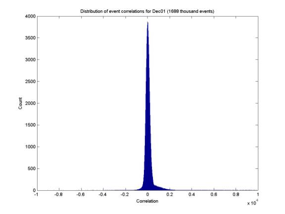
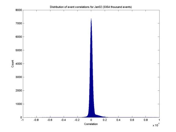
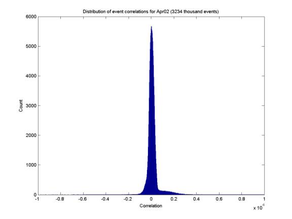
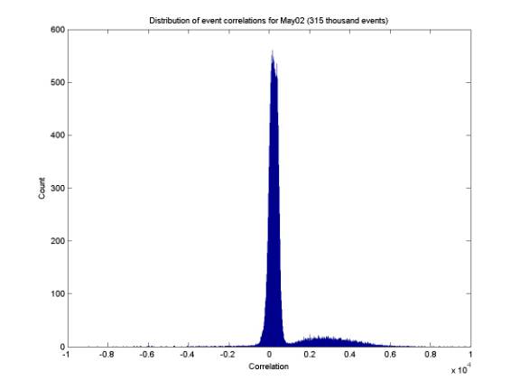
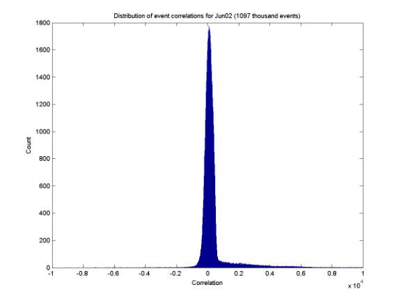
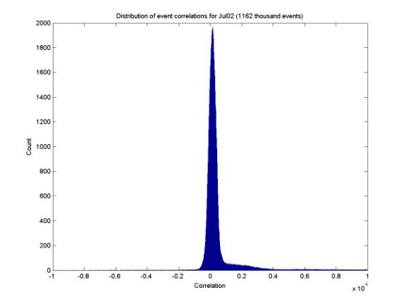
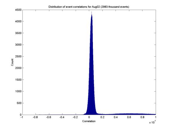
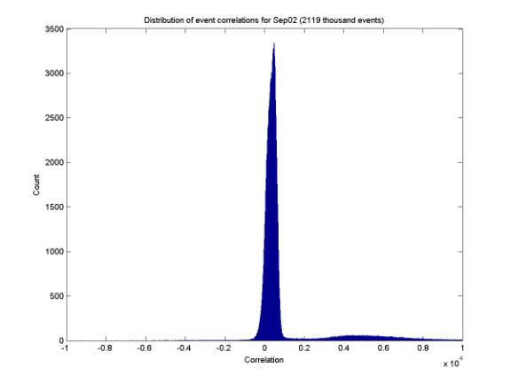
For every event, the cross talk was removed (a constant ratio of 6% was assumed), and then the correlation (sum of 21 pairwise correlations) between channels was calculated. The plots below give the distribution of correlation values for each month. Before the December 2001 upgrade, there are many events of high correlation (caused by 60 Hz line noise). After the upgrade we only plot events of code 1 and 2 (ie those that passed both triggers). Unfortunately there are still some of high correlation because the algorithm that calculated correlation offline for these plots was the correct one but the online algorithm used for several months had a small bug (fixed in ~ Sep 2002). The online algorithm is now exactly the same as the offline.


10/17/02
Correlation of code 2 events
correlationDistCode2.m
plotCorrelationDistribution.m
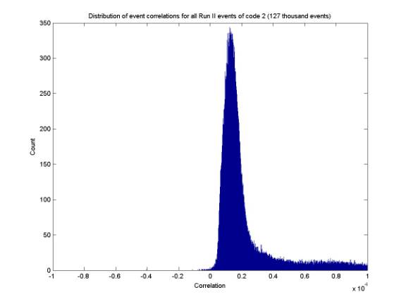
The plot below gives the correct (offline) value of the correlation of all code 2 events from Run II (events that were rejected by trigger level 2)
10/17/02
Channel indexing
checkChannels.m
All events starting at the beginning of 12/22/01 have channel indexing from 1 to 7 (checked with checkChannels.m – there are no trchan’s = 0 in event lists). Prior to that date, most indexing is from 0 to 6, but there appear to be some times during development when indexing was from 1 to 7.
10/17/02
Daily event rates by channel
eventsPerDayByPhone.m
plotEventsPerDayByPhone.m
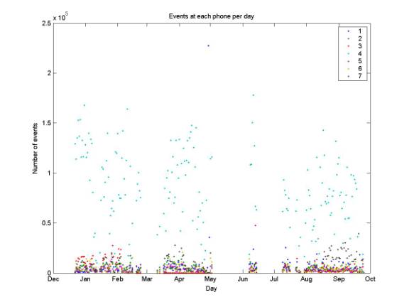
The plot below gives the daily rate of events at each phone for Run II. Note how much phone 4 dominates due to improper gain calibration. Phone 1 dominated once when the post-amp dominated before being taken off line. The table gives overall percentages of events at each phone.
10/21/02
Organization of data
From the beginning of data taking until the December 2001 upgrade (all of Run I), data were taken at Site 1, copied to CD, and shipped to Stanford on CD. A total of 46 CD’s were created. A small part of the data from these CD’s was not part of the data repository on erinyes. All data were copied from the CD’s to erinyes and the CD’s were then thrown away because they are very slow and tedious to deal with. Backups can be maintained on hep and hep26 (the PC). There is one exception: AUTEC Data CD 10 was corrupted and data cannot be read from it – it has been saved in case a method is found to restore the dat.
10/24/02
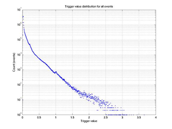
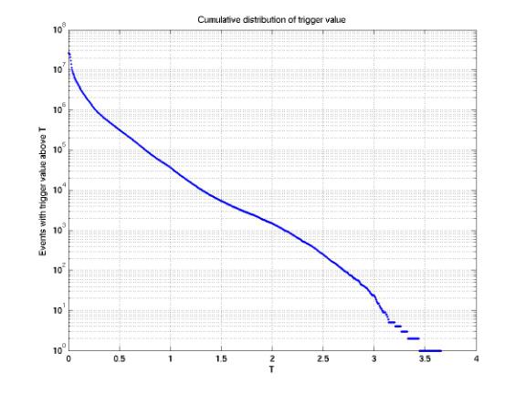
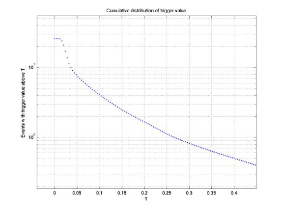
Distribution of triggering values
trvalHistograms.m
plotTrvalHistograms.m
The first plot below is a histogram of triggering value for all 26 million events. The second plot is a cumulative histogram (filter value vs. # of events above that filter value). The 3rd and 4th plots are closeups of the 1st and 2nd. All plots are only good as order-of-magnitude estimates, as the phone gains have not been properly accounted for and vary over a factor of two. Note that we could roughly reduce the event rate by an order of magnitude by raising the threshold by a factor of 3. This would result in a factor of 3 higher energy threshold, or we could maintain the same energy threshold by having a string spacing 1/3 as large.

10/24/02
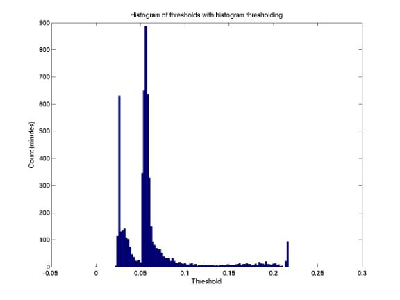
Histogram thresholding
plotThreshold.m
The first plot below gives the threshold for each minute from histogram thresholding, for the data that we have from histogram thresholding (with all phones coupled – we do not yet have data for histogram thresholding with phones decoupled). The second plot gives the distribution of threshold values, in units of the threshold step size (0.002). Note the two different running environments.

10/24/02
Distribution of filter values
hourlyFilterHist.m
plotHourlyFilterHist.m
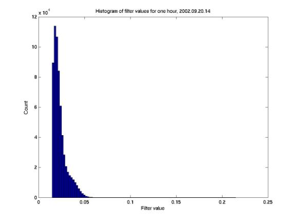
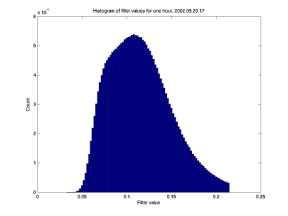
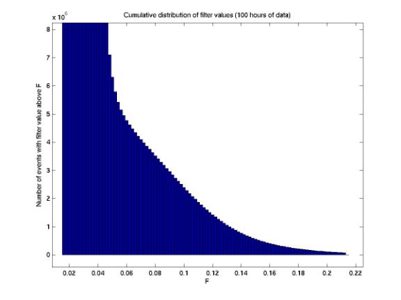
From 9/20/02 to 9/27/02 we ran with histogram thresholding with all phones coupled. An all-channel histogram is written each minute. The first plot below is a typical histogram summed over an hour of data. The second plot is an anomalous hourly histogram.
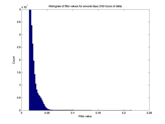
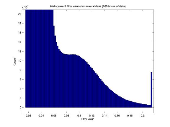
The first plot below gives the minutely histograms summed over all data
available from this period (100 hours total). The second plot is a
close-up of the same distribution. The third plot gives the cumulative
distribution. On first thought, if the low-level distribution were
constant, we could maintain a constant high threshold, eg 0.2. We would
then have a very low rate. However the 3rd plot below
indicates the rate above a high constant threshold is still high (105
samples / 100 hours = 1000 samples / hour = 17 samples / minute). It is
likely better to have a mid-range threshold (~0.1) and turn the detector off
when the rate is too high. We might be able to cut a large portion of
events above this threshold by simply turning off the detector for ~1-50 % of
the time.
10/24/02
Livetime vs. threshold
plotThreshold.m
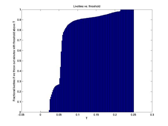
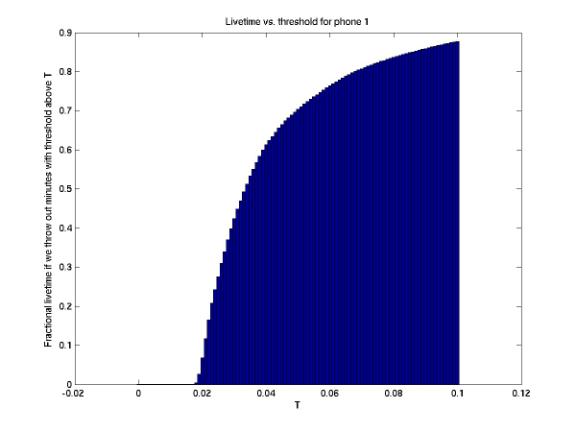
The first plot below is a cumulative histogram of threshold from the histogram thresholding algorithm. It can be interpreted as follows: We can throw out all minutes of data with threshold above some value T. We’re then left with a fraction of the livetime we had previously. The first plot below shows that we can throw out roughly all minutes with threshold above 0.05 and still have half of our livetime. We could then throw out all events with triggering value below 0.05 (taken during minutes with threshold below 0.05) and consider ourselves to be a constant-threshold detector that is turned off ½ of the time due to noisy conditions. We need more statistics to see this plot over all times of day and all times of year. But in the first plot below, the ideal location is actually the top of the near-vertical curve, before the rolloff. We then have a low threshold (~0.06) and a high livetime (~ 80 %).
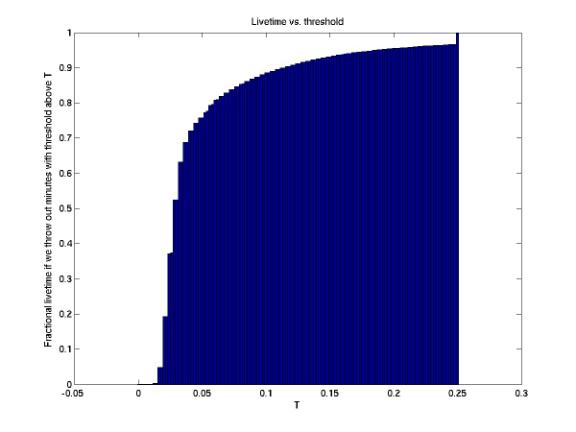
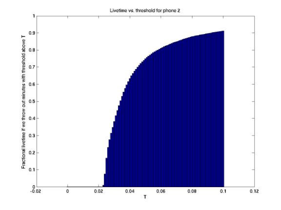
The second plot gives the same distribution for all Run II (Dec 22 2001 on) data. We see that we can eliminate all minutes with threshold above 0.05 and retain 75% of our livetime. This is very good. We can then rethreshold those minutes with threshold below 0.05, and only consider events with trigger value above 0.05. We will then have all events of filter value 0.05 or higher, taken with a detector that is regularly turned on and off depending on noise conditions.
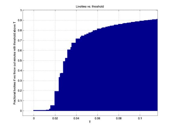
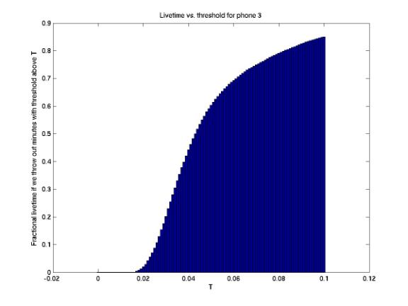
The third plot gives the same distribution for all Run I and Run II data. We started from 2001.08.23 – 2001.08.20-22 had a bug in the thresholding algorithm that caused very large thresholds. Cutting at a threshold of 0.05 gives maintains a 75% livetime.
10/25/02
Eliminating minutes with high threshold
quietMinutes.m
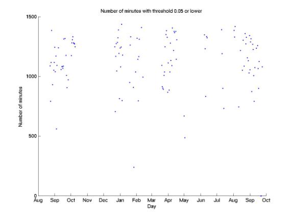
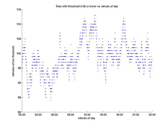
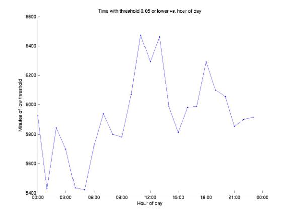
We have 128 days for which data were taken during all 1440 minutes. For each of these days, we have removed those minutes with threshold greater than 0.05. The first plot below shows the number of minutes remaining for each day once this is done. There are two days in September for which 1440 minutes of data were taken but none of the minutes had a threshold below 0.05. The baseline of thresholds for those minutes was abnormally high. The second plot gives, for each minute of the day, the number of days which had a threshold below 0.05 for that minute. The third plot gives the same data for each hour of the day. Noon to midnight appears to be less noisy than midnight to noon. When this cut was made, 128 * 1440 = 184,000 minutes of livetime were reduced to 142,000 minutes, or 77% of the initial livetime. We have a total of ~300,000 minutes of data on disk. There are 17 million events in the 128 full days, and 13 million (76 %) remain after eliminating noisy minutes.
10/25/02
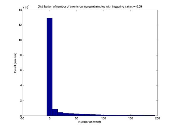
Restriction to events with triggering value >= 0.05
plotRemoveLowTrvalEvents.m
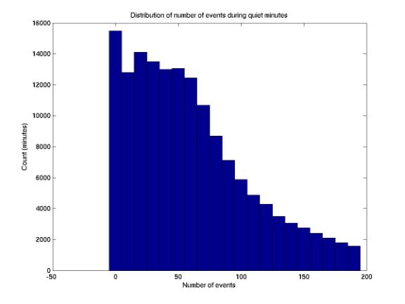
Once we’ve eliminated minutes with threshold above 0.05, we have 173,000 minutes of data containing 13 million events. We can then eliminate those with trigger value below 0.05, leaving 5 million events. We now have a constant-threshold detector that is turned off when conditions are too noisy. The distribution of events per minute is given in the two plots below, before and after removing low - triggering value events. Note that after eliminating events, 130,000 minutes have no events at all. We can then run at 50 % of the time with a threshold of 0.05 and have no events! So with criteria for background rejection (including coincidence) we could have a lower threshold.
10/31/02
Data compression for backup
zipData.m
checkData (shell script)
All data have been zipped using zipData.m (with the exception of the ~25 GB day 2001.07.26, which was split into 3 zip files because zip has a file limit of ~ 10 GB uncompressed - perhaps corresponding to ~2 GB compressed, which would be the limit due to 32-bit integers). There is a useful shell script, checkData, which verifies zip files relative to initial files (both number of minutes per day and total uncompressed size). This script has been run on all data except 2001.07.26
11/01/02
Distribution of thresholds with decoupled histogram thresholding
plotThresholdDecoupled.m
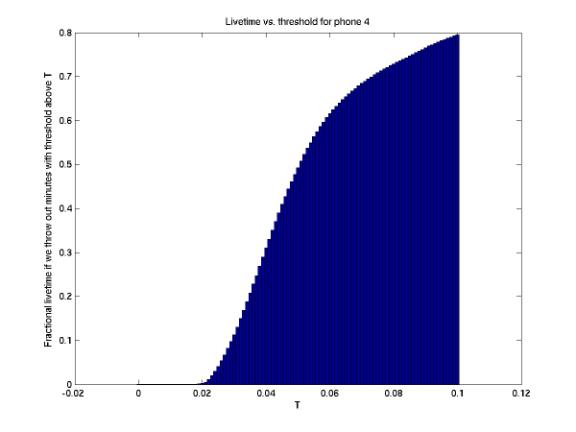
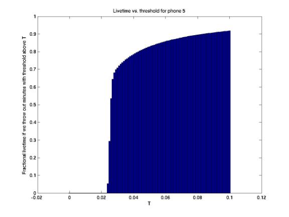
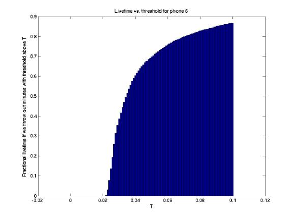
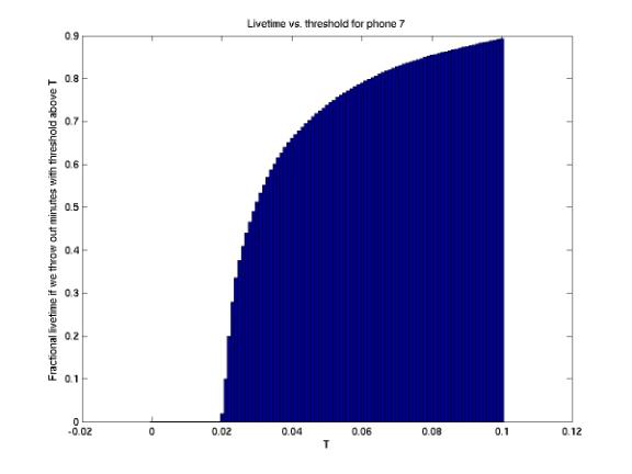
The plots below give the cumulative distribution of threshold for each channel, using decoupled histogram thresholding (every phone has its own threshold each minute that is determined from a histogram of filter values built the previous minute). The plots were determined from all decoupled histogram thresholding data we have (568 hours of data from 9/27/02 to 10/21/02).
11/1/02
Event rates at each phone
eventsPerMinutePerPhone.m
plotEventsPerMinutePerPhone.m
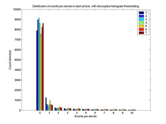
The first plot below gives the distribution of events per minute at each phone, with file format 6 (decoupled histogram thresholding and bug fixes from format 5). 10,842 minutes of data are included, from 10/11/02 to 10/21/02. Note that the distribution does not vary from channel to channel. Also, we are dominated by minutes with zero events. This is good; it means we have a low background. The mean rates (events per minute) are as follows:
Phone Rate
1 3.8
2 2.6
3 3.7
4 4.2
5 3.8
6 3.9
7 2.6
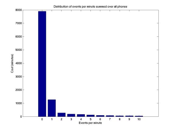
We have a target of 10 events/minute/phone. It is unclear why the means are lower. Perhaps there is a small systematic error in the online code. However, is is not very important as the histogram thresholding typically chooses a value from a very sharp curve, so having a target of 1, 10, or 100 events per minute would result in very similar thresholds. The second plot below gives the distribution of total events per minute (summed over all phones). Note that ~ 80 % of minutes have no events.
11/1/02
Threshold vs. event rate
plotThresholdVsNumEventsDecoupled.m
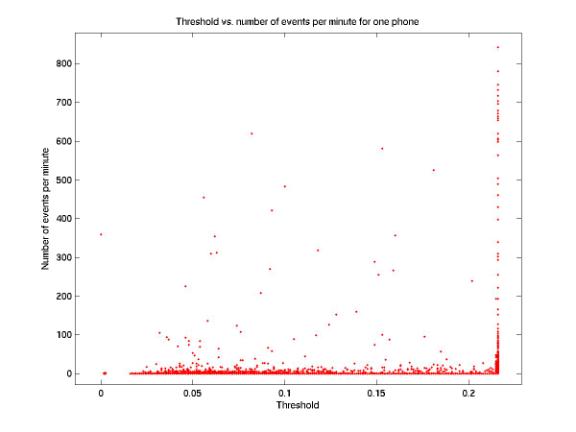
The plot below gives, for phone 3, the threshold vs. the number of events each minute. Online, the filter value histogram maxes out at 0.216, so our threshold cannot rise above this value. Therefore we are typically swamped when the threshold is this high. Offline, events taken during minutes with a threshold of 0.216 should be neglected (they are taken during high noise anyway). It might be worth histogramming up to 1 or so in the next online code. There is also a strange occurrence of minutes with threshold below 0.016, which should be the minimum.
11/1/02
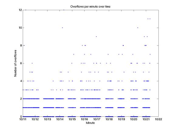
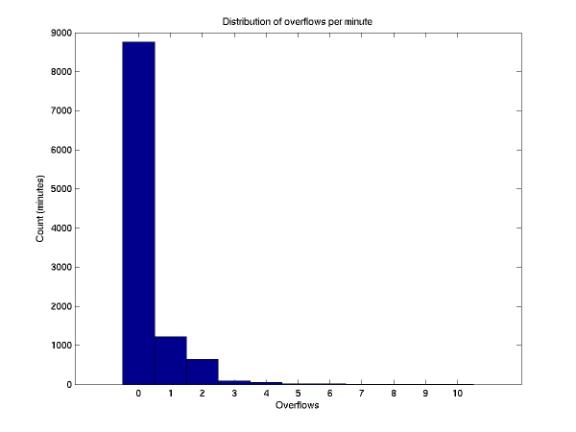
Overflows
olmLookupTable.m
plotOlmLookupTable.m
The plots below summarize the rate of overflows with the new online code (10842 minutes of data analyzed). Note 75% of minutes have no overflows.