Log 6

Justin Vandenbroucke

justinv@hep.stanford.edu

Stanford University

12/5/02 – 12/12/02

This file contains log entries summarizing the results of various small subprojects of the AUTEC study. Each entry begins with a date, a title, and the names of any relevant programs (Labview .vi files or Matlab .m files – if an extension is not given, they are assumed to be .m files).

12/5/02

Monte carlo acceptance calculation

calcAcceptanceMC.m

plotAcceptance.m

I switched from a part-grid, part-monte carlo calculation of acceptance to entirely monte carlo. The radiation pattern (a 3D field of pressure signals with appropriate amplitude)) is determined by the initial neutrino energy, E₀. A single-phone filter threshold then determines a detection contour within this pattern. The number of phones that lie within this contour (the number of phones hit, n) depend on the neutrino path direction and the location of the interaction (5 coordinates: x, y, z, theta, and phi). For a given E0 and n, the acceptance is the volume of points in this 5D space that result in n or more phones hit. We can determine values for n = 4, 5, 6, and 7 simultaneously by generating random 5D points and counting the number of phones hit. For the plots below, 10⁶ points were generated, taking ~ 1 hour for each value of E₀. The first 11 plots below are all for E₀ = 6e20 eV, the highest value yet used.

Points must be chosen from very different ranges for n = 1, 2, or 3. For n=1 we can have the interaction far above the plane and still hit one phone, with the radiation plane perpendicular to the detector plane. Similarly for n=2, as long as the plane of the radiation intersects 2 phones. Similarly for n=3, because there are 3 spokes that have 3 colinear detectors. For n=4, however, the radiation plane must coincide with the detector plane, so our polar angle is restricted to being very nearly zero. We require n=4 for coincidence anyway, so it is unnecessary to calculate n= 1, 2, 3.

The first 5 plots below give the distribution of the points in the 5 coordinates. Phi, the azimuth angle, ranges from 0 to 360. Acceptance should be 60-degree periodic in phi, because the detector has 6-fold radial symmetry. Theta, the polar angle, is chosen from 0 to 1 degree (the abscissa in plot 2, mislabeled as degrees, is in radians). Nonzero acceptance is expected to be within this range. Theta is chosen not from a uniform distribution but from that of points chosen randomly on an actual sphere (ie it incorporates a spherical metric). See http://mathworld.wolfram.com/SpherePointPicking.html. Near theta=0, the distribution is nearly linear. x, y, and z are chosen from uniform distributions with ranges chosen appropriately from the dimensions of the radiation pattern for the E₀ in question.

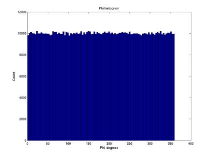
Figure 1

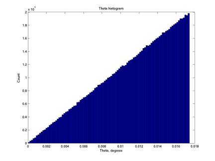
Figure 2

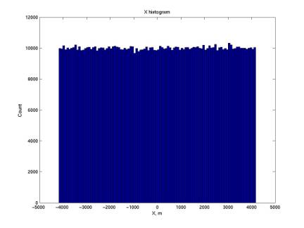
Figure 3

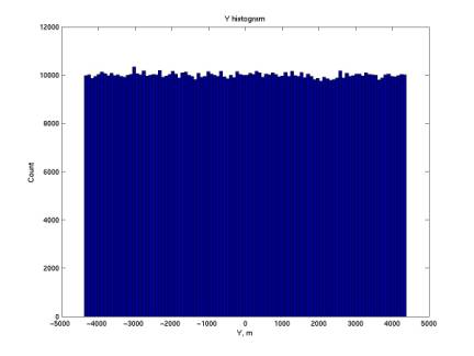
Figure 4

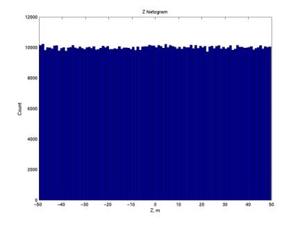
Figure 5

The plot below gives the distribution of n, the number of phones hit.

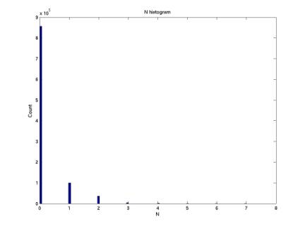
Figure 6

Once enough points have been determined for a given energy, we can calculate acceptance for each n. Count the number of points that resulted in n or more phones hit; call this N_good. Let N_total be the total number of points generated. Let A_total be the total acceptance range we are integrating over,

A_total = 8 * X_max * Y_max * Z_max * 2p * (1 – cos(U_max)). Then A = A_total * N_good / N_total.

The two plots below give the convergence of our calculation as more points are generated. The second plot is a close up of the n=7 case. It is very rare that all 7 phones are hit, so Ngood is very small. The strange feature of large jumps upward followed by smooth declines is understood by considering that the 7-phone events are rare, so acceptance jumps up when each new one occurs and then slowly decreases as more events are generated that do not hit 7 phones.

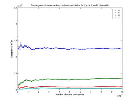
Figure 7

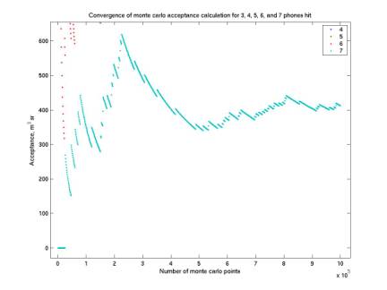
Figure 8

The plots below give acceptance as a function of zenith, azimuth, and height above detector. For zenith, the curves increase at first because binning is by constant theta, not constant solid angle. They then decrease as the radiation plane leaves the detector plane. Note that we are only sensitive to zenith below 0.5 degrees.

The absolute magnitude for the azimuth and height plots are not correct here but have since been corrected.

We expect the curves for azimuth to have a slight 60-degree periodicity that is difficult to observe here. It may be that the periodicity is very small.

The height plot is not centered on zero because the z coordinate of the radiation pattern is not at the radiation maximum but at the neutrino interaction point.

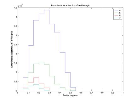
Figure 9

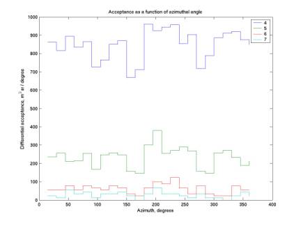
Figure 10

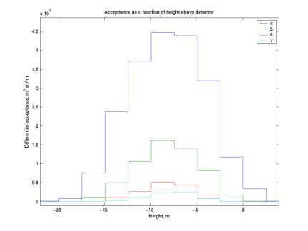
Figure 11

12/9/02

Acceptance vs E₀

calcAcceptanceVsE0.m

plotAcceptanceVsE0.m

The plot below gives acceptance as a function of neutrino energy for n=4,5,6,7. Our acceptance is zero until ~ 3-4 e20 eV because the radiation disk radius is too small to possibly hit 4 phones – it must be at least ~ 1.3 km (see log 5 for E₀ vs R).

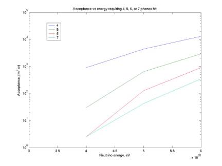
Figure 12

12/11/02

Weird radiation pattern

plotDetectionVolumeRect.m

The first plot below shows detection curves for 1e20 eV to 6e20 eV, enclosed within the grid of radius 3 km. When the grid was extended to 6 km and curves were plotted up to 12e20 eV, the second plot below emerged. The scalloping and islands are strange and unexpected. I think it’s possible that the pattern is an artifact of sampling. Nikolai’s code generates signals sampled with dt = 1e-6 s, but I then resample it with dt = 5.6e-6 to match our experimental conditions.

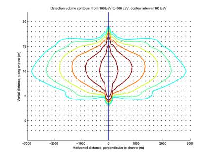
Figure 13

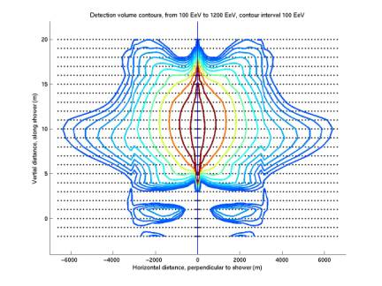
Figure 14

12/12/02

Weird radiation pattern continued

plotDetectionVolumeRect.m

For the plot below, Nikolai’s code was run sampling with dt = 5.6e-6, so no resampling was necessary. The difference between these curves and those above indicates that it is indeed a sampling problem. I’m trying now to sample with a dt 4 times smaller. I can then sample at 5.6e-6 s by taking every 4^th sample. There are 4 different ways to do this. I imagine each will result in a different scalloped pattern. Hopefully by averaging the 4 for each grid point we will get smooth non-scalloped curves. These will represent the average case. For each experimental signal that occurs, our detection volume could be larger or smaller depending on the offset of our sampling relative to the signal.

These curves are the basis for our acceptance calculation, so we’d like to get them right.

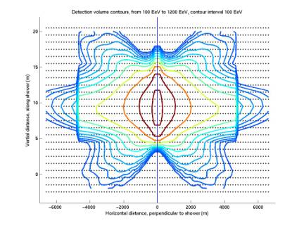
Figure 15

12/12/02

Neutrino-nucleon cross sections

sigmaEstimate.m

plotSigmaEstimate.m

The two plots below give estimates of the cross section for our experiment. We will fold this into our acceptance calculation to have acceptance in cm^2 sr rather than cm^3 sr. The estimates are calculated from a power law valid for 10¹⁵ eV to 10²¹ (Gandhi and Quigg, hep-ph/9512364). The first plot shows sigma for this whole range; the second shows it for the energies for which we’re currently calculating acceptance.

There’s a series of Gandhi and Quigg papers that analyze up to 10^21 eV and give tables for each order of magnitude. We would like a table that extends an order of magnitude or so farther and has better resolution than one order of magnitude.

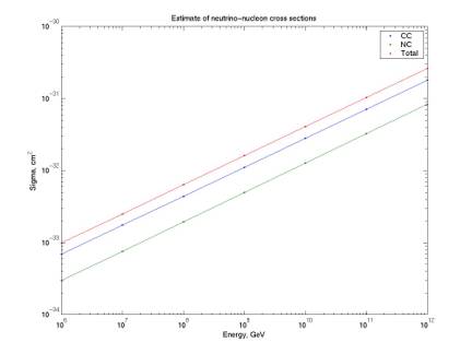
Figure 16

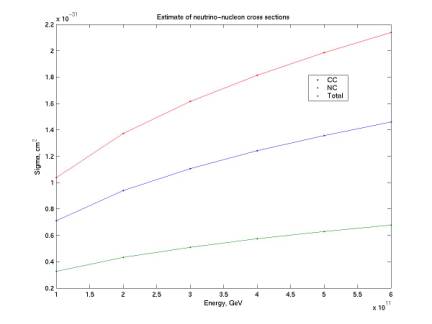
Figure 17

12/12/02

Conversion of acceptance to standard units

plotAcceptanceVsE0.m

The three plots below show the conversion of acceptance from the easiest units to calculate to standard units. We initially calculate in (m^3 sr) in our monte carlo code. We can then convert this to (nucleons sr) by multiplying by the nucleon density of water. This is Avogadro’s number, 6.022e23 nucleons/cm^3, or 6.022e29 nucleons/m^3. Nucleons are not typically shown as a unit but we retain them here for clarity. Finally, in the third plot we fold in the cross section as shown in the plot above. We now have acceptance in its standard form (nucleons sr cm^2).

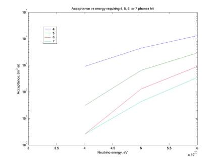
Figure 18

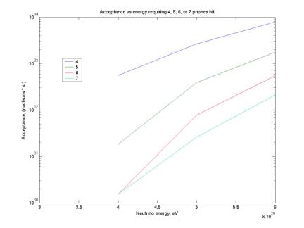
Figure 19

Figure 20