Log 8
Justin
Vandenbroucke
justinv@hep.stanford.edu
Stanford
University
1/10/03 –
1/27/03
This file contains log entries
summarizing the results of various small subprojects of the AUTEC study. Each entry begins with a date, a title,
and the names of any relevant programs (Labview .vi files or Matlab .m files –
if an extension is not given, they are assumed to be .m files).
1/10/03
Check of completeness of derived data
We
must check that all relevant programs have been run on all data available from
Run II. Each program named prog.m typically
outputs a file named prog.mat for each hour
of data. Below we count the number
of prog.mat hourly files present for each prog. We use countFiles.m to count the prog.mat files. According to countHoursOfData.m applied to run2HourRange(), we have 3567
hours (149 days integrated) of data taken during the 6657 hours from 2001.12.22
to 2002.09.25.08. Below is given
the number of hourly files for each prog.mat:
3567
eventListComp
3567
coincidenceEventListsComp
3567 bestCEL
3567 hyperbolateAll
It is clear that we have completely run the relevant
programs on all data.
1/24/03
Error in detector plane determination
detectorPlane.m
In
Log 5 (11/4/02) I determined the least-squares plane of the detector (along the
sea floor, tilted from the horizontal) but it turns out the algorithm was
finding a local minimum. The plane
is actually tilted at 0.6 degrees, not 0.1 degrees as reported previously. The phones span only 5 m perpendicular
to the plane, not 17. The heights
above the detector are given in Table 1.
Table 1
The
plane normal is 0.6 degrees from the vertical (corresponding to a 1% grade) and
7 degrees East of North.
1/24/03
Transformation to
detector plane coordinates
tiltedPhones.m
We have been using a coordinate system with origin at the sea surface directly above the central phone, with (x, y, z) = (N, E, down). This is awkward for many purposes. tiltedPhones.m applies the following rigid transformations to produce coordinates aligned with the detector, right side up, with the origin in the detector plane:
1) Translate vertically so the central phone is at the origin.
2) (x, y, z) = (N, E, down) ® (x, y, z) = (E, N, up)
3) Rotate z axis to the plane normal.
4) Translate along the new z axis (perpendicular to the plane), so the origin is in the plane rather than at the central phone.
Below the detector is plotted looking along each of the three axes in the new coordinate system.
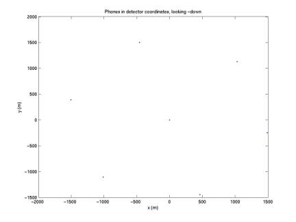
Figure 1
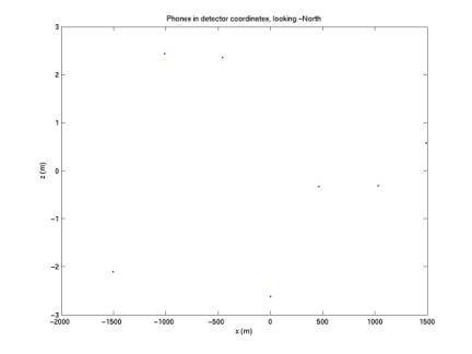
Figure 2
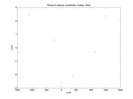
Figure 3
1/24/03
Corrected contours
AUTEC_analysis/acoustic/acousticRect (executable, compiled from my modifications to Nikolai’s acoustic simulation code, version 1)
AUTEC_analysis/acoustic2J/acoustic (executable, compiled from my modifications to Nikolai’s acoustic simulation code, version 2 )
PlotDetectionVolumeRect.m
Nikolai wrote a new version of his acoustic simulation code, and I modified it. The first plot below is generated from rect’s 42-47, which were generated by the original version. The second plot is from rect’s 66-71, which were generated by the new version. The new one is missing the mysterious structure we’ve been wondering about. The new version also ran much faster (~ 1 hour compared to ~ 8 hours). These differences could be due to Nikolai’s new integration algorithm, or differences in the input parameters, or a change I made to the precision of the output files (I had been writing 6 digits past the decimal in the mantissa, rather than 16).
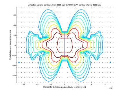
Figure 4
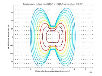
Figure 5
1/27/03
Contour mystery explained
plotDetectionVolumeRect.m
The strange structure we were seeing previously was due to a bug in the old version of acoustic. In acoustic2, Nikolai changed an occurrence of (z2-z1) to (z2+z1). When I change it back and leave everything else unchanged, the code with the bug (rect’s 96:101) generates the scalloped contours and the correct version (rect’s 66:71) generates smooth contours.
1/27/03
Constancy of contours
PlotDetectionVolumeRect.m
The contours are quite constant under changes to the input parameters h, r[i+1]/r[i], dz, and integration algorithm. The less-precise versions run significantly quicker.
1/27/03
Acceptance vs. energy for various detectors
plotAcceptanceAllArrays.m
Using Monte Carlo integration over 3 spatial coordinates and 2 angles for shower location and orientation, we’ve determined the acceptance as a function of energy for our detector as well as for two possible future detectors. In the plot below, “Current” denotes our detector, with exact hydrophone coordinates (ie it includes the effects of not all phones being coplanar and of the detector being 1 degree from the zenith). “Cubic100” is a cubic array of 1000 phones (10 x 10 x 10), with spacing 100 m. “Cubic1000” is a similar array with spacing 1000 m (ie it is optimized for higher energies). Note that it is similar in shape to the curve for our current detector, with higher magnitude. By increasing the number of phones by ~ 2 orders of magnitude, we get 5 orders of magnitude higher acceptance. This is because the cube has many more planes that can coincide with the plane of the acoustic radiation, and the acceptance is over all 90 degrees of zenith rather than being limited to a few degrees of zenith.
All acceptances shown are calculated requiring 4 phones hit. Similar curves can be determined requiring more phones hit.
All acceptances are calculated with a threshold of 0.05.
The “Current” and “Cubic100” arrays have zero acceptance below ~ 4e20 eV because below that energy the radiation disk is not wide enough to hit 4 phones.
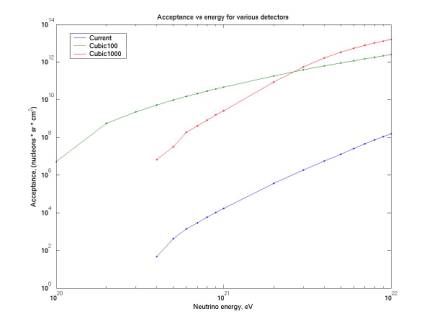
Figure 6
1/27/03
Differential flux limits using various flux models
calcLimits.m
The plot below shows our differential flux limit assuming the flux follows a power law of index gamma, for various gamma’s. The second plot below (from John Learned’s talk at Fermilab) gives the same quantity (I believe) for other experiments and theories. The third plot below gives limits from the RICE experiment (also from JL’s talk).
If I’m using it correctly, the flux model tells us how to divide our ~ 1 event among the various energies. I assume that we have seen of order 1 event, so 1 = N = integral(X * phi * dln(E/eV), E1, E2). Here phi(E) = alpha * E ^ (-gamma) in cm^-2 sr^-1 s^-1 / ln(E/eV) and X(E) is our exposure in cm^2 sr s. We than solve for alpha given various values of gamma and our flux limit is phi(E).
I’m not sure I’m doing this correctly. For one thing, by this method gamma exactly determines the shape of our limit. This is consistent with the RICE curves but not with the other curves (second figure).
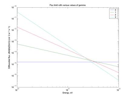
Figure 7
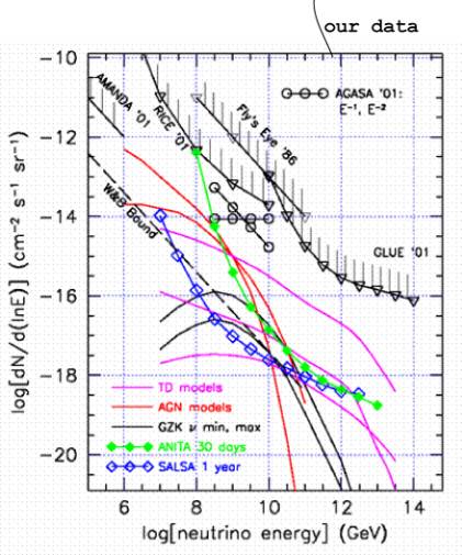
Figure 8
Figure 9
1/27/03
Flux limit as inverse exposure
calcLimitsOld.m
The old method of calculating our flux limit was simply to take the inverse of the exposure. This had a shape that seemed to be more naturally determined by our data, but I don’t know how to turn it into a differential flux as it should be. This flux has units cm-1 sr-1 s-1 and is not differential in energy.
The method is as follows: first we determine our livetime at each threshold, shown in the first figure below. We then determine the exposure with each threshold, shown in the second figure below. Note that the higher the threshold his, the higher the energy necessary to have positive acceptance. To find the total exposure we then sum the independent exposures at each threshold. In the second figure below, the top curve is the total exposure. The second (green) curve is for threshold 0.02. The next two curves, red and blue, are for thresholds 0.03 and 0.01.
We see that 0.01 and 0.02 dominate the sum. So we can neglect all exposure with threshold above 0.025 (the 0.02 bin includes 0.015 to 0.025). We consider the minutes with these thresholds too noisy to be useful. We can then eliminate all events recorded during these noisy minutes without significantly affecting our flux limit.
The third plot below gives our flux limit assuming it is simply the inverse of our total exposure.
The second and third plots will be extended beyond 2e21 eV pending more Monte Carlo calculations of acceptance at high energy.
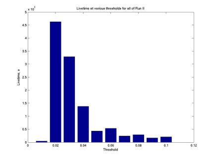
Figure 10
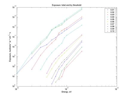
Figure 11
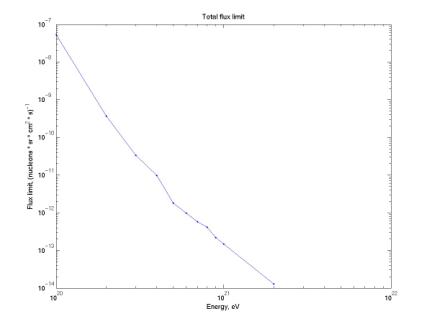
Figure 12
1/27/03
Systematic
rejection of neutrino candidates
My initial
strategy was to determine all combinations (groups of 4 single-phone events
that form a diamond of nearest neighbors and occur within speed-of-sound
limits), then raise the threshold of each minute independently until no
combinations remain. However this
would reject all neutrinos if any were present and would result in a flux
estimate much lower than the correct value.
Instead I
maintain a variable threshold (first determined online and adjusted offline if
necessary) that is a multiple of a fixed step size and results in ~60
events/minute. This is adjusting
the threshold based on a bulk statistical noise rate and should not be affected
by individual events, including neutrinos.
After
doing this, candidate neutrino events remain. We must reject them property by property:
1)
Event depths
eventDepths.m
Of 707,066 total
4-phone combinations occurring in 3567 hours of livetime, only 3970 occur on
the bottom 100 m of the sea. It
must be within of order this depth (and close to vertical incidence) in order
for the flat disk of radiation to overlap with the detector and trigger
multiple phones.
2)
Thresholds
botThresholds.m
Minutes with threshold above ~0.025 contribute negligibly to our flux limit, because our acceptance (~ effective volume) is very low with these thresholds. Therefore we can simply consider our detector to be turned off during these minutes due to high noise levels and can ignore events that occurred during them. Doing so rejects 3928 of the 4158 total combinations, leaving 220.
3)
Nikolai parameters
botNikParams.m
Of the 220 remaining events, only 138 have ntyp < 4, as all simulated neutrino events do (see p. 46 of Nikolai’s University of Hawaii talk, http://hep.stanford.edu/neutrino/SAUND/uhtalk.pdf)
4)
Waveforms
plotCandidates.m
By plotting all 138 one-by-one, we can visually reject diamonds, pings, correlated noise, and spikes. I’m working on writing code that will reject these, which should be more objective than visually inspecting each waveform. This leaves us with only two events (numbers 1 and 104 of the 138), shown in the two plots below. They both have a shape consistent among all 4 phones and are both ~3-polar. These ~3-polar events occur regularly throughout the data. It is unclear if the original acoustic signal was ~3-polar or if they could have been bipolar (ie neutrino-shaped) and then transformed by the microphones + amp (including filters).
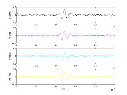
Figure 13
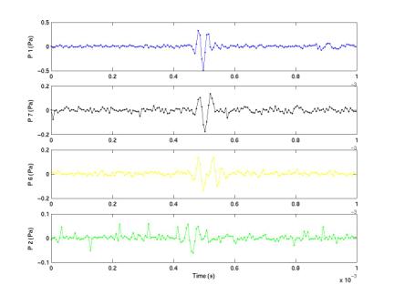
Figure 14
1/27/08
Measurement of cross-section from events
With enough confirmed neutrinos, an experiment like ours could measure the neutrino-nucleon cross section. We would start by binning events by energy. We would then determine, for each energy, the flux as a function of zenith angle. Given the overburden of earth/water as a function of zenith (from 0 to pi) we would then convert this to flux as a function of overburden. Assuming isotropic flux incident on Earth, we expect this to be phi = phi0 * exp[-L/Lint], so we fit for phi0 and Lint. This is done for each energy, giving us Lint(E). This is then converted to sigma(E).