Log 9

Justin Vandenbroucke

justinv@hep.stanford.edu

Stanford University

1/30/03 – 2/3/03

This file contains log entries summarizing the results of various small subprojects of the AUTEC study. Each entry begins with a date, a title, and the names of any relevant programs (Labview .vi files or Matlab .m files – if an extension is not given, they are assumed to be .m files).

1/30/03

New contours for extreme size ranges

plotDetectionVolumeRect.m, for mode = extraLarge and tiny

The two plots below extend the range of our acoust radiation detection contours for various energy values. All contours are for threshold 0.05 (roughly the mean), but we only include up to 0.02 in our flux limit calculation.

The first plot spans 40 km radius and 400 m width, and gives energy contours from 10²² eV to 10²³ eV.

The second plot spans 300 m radius and 10 m width, and gives energy contours from 2 x 10¹⁹ eV to 10²⁰ eV.

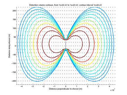
Figure 1

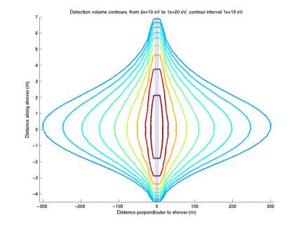
Figure 2

1/30/03

Large-scale bathymetry within a few km of our detector

site3Bathymetry.m

The plot below gives depth contours for the phones surrounding our detector. Jack sent me the coordinates by email on 1/28/03. He’s since also sent coordinates for phones to the East and South, but I haven’t yet plotted them.

The curves are useful for giving the general slope of the sea floor, but tell us nothing about how rough it is on a smaller scale. There could still be bumps of up to a couple dozen meters spanning ~ 1 km. These could block a significant amount of our effective volume.

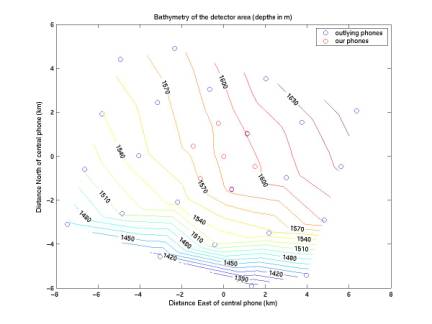
Figure 3

2/2/03

New acceptance curves

plotAcceptanceAllArrays.m

The plot below gives acceptance curves for our current detector as well as for 3 possible cubic configurations of 10 x 10 x 10 phones, with phone spacing of 100 m, 1000 m, or 10000 m.

The acceptance is for a 0.02 threshold, the low (quiet conditions) threshold used most for our flux limit.

The lower ends of the curves are the lowest energies for which we have nonzero acceptance for each array. This is determined by the requirement that we hit 4 phones: below this energy the acoustic radiation does not span enough area to cover 4 phones, even in ideal orientation. The upper ends extend indefinitely, as long as we have infinite water.

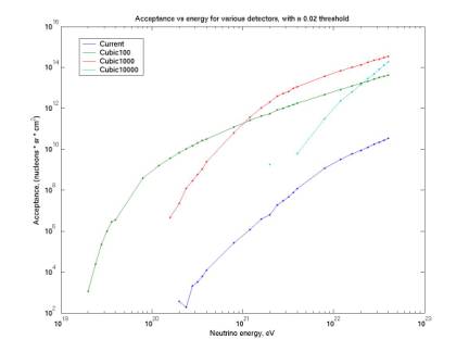
Figure 4

2/2/03

Depth profile

depthProfile.m

The plot below gives the distribution of reconstructed event depths (perpendicular to the sea surface, not the sea floor / detector). All combinations are shown, most of which are not physical (because of our unstable event rate, we often have many combinations of events within the coincidence window). The non-physical events extend to large tails on both sides. The sea surface is at 0 m, the sea floor at 1600 m. The distribution is symmetric about the sea floor because the reconstruction algorithm cannot distinguish between a location and its mirror about the sea floor (because the detector is planar). Both points are solutions to the hyperboloid intersection. There is an excess of events at the sea surface, perhaps due to surface noise (wind, waves, rain).

The sharp decrease at the sea floor is disturbing because this is our effective volume. I see threee possible explanations: (1) blocking by hills of the floor; (2) systematic error in the hyperboloid intersection method; (3) an actual decrease in (biological?) noise sources.

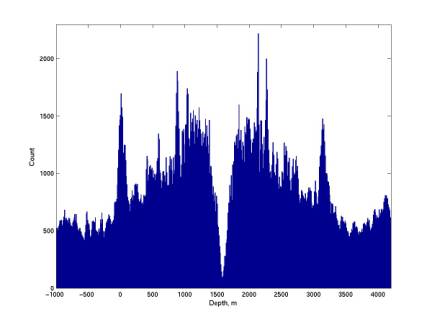
Figure 5

2/2/03

New acoustic radiation contours

plotDetectionVolumeRect.m, mode = small02

The contours below are for a threshold of 0.02 (not 0.05 as all others are). Contours are given for 10²⁰ to 10²¹ eV, our most interesting range.

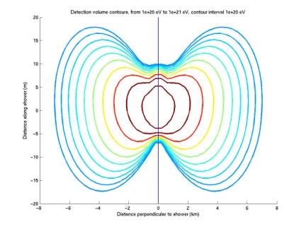
Figure 6

2/2/03

Examples of rejected events

plotCandidates.m

The events plotted below are examples of our 138 candidates within 100 m of the sea floor, during minutes with threshold < 0.025, with characteristic number of periods < 4. Signals are given for 4 channels, with the channel number on each y axis. In the title bar are given date, time of day, and coordinates in m (x, y, h) = (East of center phone, South of center phone, height above sea floor).

The three events are of the following types: diamond (dolphin?), ping (freq ~ 10 kHz), spike (single-sample displacement).

Note: often one of the 4 signals is distinguishable of one of these types and another is of another type. These events are rejected, even if one type is tripolar (consistent with neutrino waveform), because they are considered to be random coincidences not corresponding to the same original source.

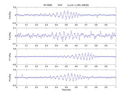
Figure 7

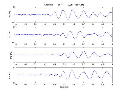
Figure 8

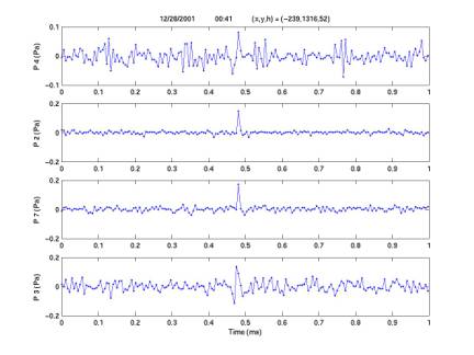
Figure 9

2/3/03

Radiation dimensions as a function of energy

calcDiskDims.m

plotDiskDims.m

The four plots below give the dimensions of the acoustic radiation for a threshold of 0.02 (Note: this is not equal to the effective volume dimensions of the detector). Height is measured along the incident neutrino axis, radius perpendicular to this axis.

The radius, and hence the volume, curve bends to a lower slope at ~ 1 km. This is presumably due to a change of radiation region relative to the source, but I have not yet squared this with Learned’s paper.

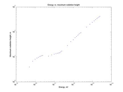
Figure 10

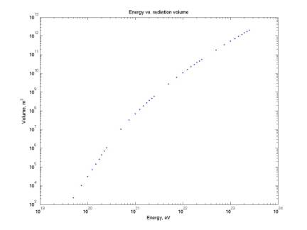
Figure 11

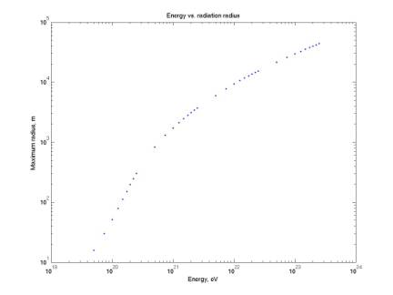
Figure 12

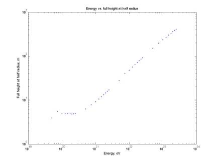
Figure 13

2/3/03

New flux limit

calcLimit2.m

The plot below gives our differential flux limit, calculated by the new method Giorgio and I agreed upon:

F(E) = integral flux = flux of neutrinos of energy > E (cm^-2 s^-1 sr^-1)

X(E) = integral exposure = our exposure for neutrinos of energy > E (cm^2 s sr)

N(E) = integral number = number of neutrinos we detect that have energy > E

Then N(E) = F(E) * X(E), so F(E) = N(E) / X(E). We can calculate F(E), and it's actually our flux limit, but it's

integral. So we just differentiate it, numerically, to get a differential flux. N(E) will be calculated from a table for Poisson rates for a given confidence level, but it does not change much, so the differential flux is phi(E) ~ -N(E) * d[1/X]/dE. Note the negative sign (the flux is actually the absolute value of the derivative, and 1/X is decreasing).

Here I have assumed N(E) is constant, N(E) = 5 for all energies. I will replace this with actual values (expected to be between 2 and 5 depending on the energy) once we are confident of our final candidates and their energies.

Our acceptance will not grow signifantly at higher energyes than 1022 eV because the effective volume hits the shore (I have allowed it to grow significantly beyond the instrumented volume for the purpose of the limit, but I would not use this volume for actual event reconstruction if events were detected within it). We need to decide exactly where to cut our volume off.

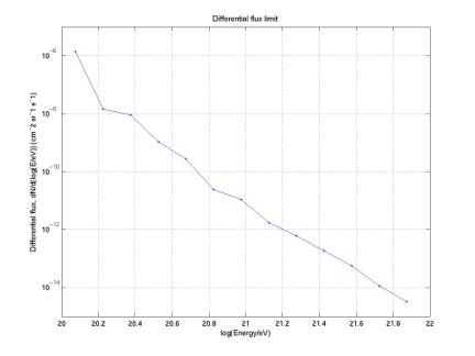
Figure 14

2/3/03

Example acceptance calculation

calcAcceptanceMC.m

plotAcceptance.m

plotAcceptanceVsE0.m

Here I walk through an estimate of acceptance at 4 * 10²¹ eV with a 0.02 threshold. It’s calculated by Monte Carlo code as follows: first we choose reasonable bounds on x, y, z, theta, and phi (theta is 0 to thetaMax, which increases with energy; phi bounds are always 0 to 360 degrees). Then we choose random random points in these 5 coordinates (points chosen uniformly in all but theta; theta chosen appropriately for isotropic flux: see http://mathworld.wolfram.com/SpherePointPicking.html).

For 4 * 10²¹ eV with a 0.02 threshold, x and y are chosen in –5000:5000 m, z in –125:125 m, theta in 0:2 deg = 0:0.03 rad). This gives a total integration volume (in the 5D coordinate space) of 2*pi*(0.03)²*(1e4 m)²*(250 m) = 10⁸ m³ sr. To convert units, we multiply by the cross section and the number of nucleons per volume: (10⁸ m³ sr) * (6e29 / m³) * (2e-31 cm²) = 1e7 cm² sr. Now in our Monte Carlo code, only ~ 1 in 10³ points in our 5D coordinate space hit 4 phones or more. So our actual acceptance for 4 phones is 1e7 cm² sr * 1e-3 = 1e4 cm² sr, which matches the value in the acceptance plot above.

2/3/03

Candidate event energy reconstruction

reconstructE0.m

I reconstructed initial neutrino energy for each of our two neutrino candidates, using Learned’s eqn. 23. Using this equation (integral of pressure-squared, scaled and attenuated properly), we get an energy reconstruction from each phone’s signal (and distance to reconstructed source). Here I report the mean and standard deviation among the four energy measurements (events are numbered within the final 138 candidates):

Candidate 1: (6 ± 4) e20 eV

Candidate 104: (4 ± 3) e20 eV