Log
10
Justin
Vandenbroucke
justinv@hep.stanford.edu
Stanford
University
2/8/03
This file contains log entries summarizing the results of
various small subprojects of the AUTEC study. Each entry begins with a date, a title, and the names of any
relevant programs (Labview .vi files or Matlab .m files – if an extension
is not given, they are assumed to be .m files).
2/8/03
Quiet livetime
quietLivetime.m
The
plot below gives the left-hand tail of our threshold livetime
distribution. These are the quietest
periods, and only these values are used to calculate our limit. Note that there are only 4 discrete
thresholds present (the thresholding algorithm steps in multiples of 0.004). For each threshold the total livetime
(summed over all minutes with that threshold) is given. The total amount of quiet (threshold
< 0.025) livetime is about 1/3 of our total livetime.
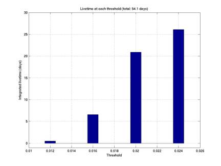
Figure 1
2/8/03
Flux limits for interactions and neutrinos
calcLimit3.m
The
first plot below gives the cross section used (an extrapolated power law from
Gandhi et al) for our neutrino flux limit.
The
second plot gives integrated flux limits, both for interactions (per unit
volume per unit time per steradian) and for neutrinos, assuming all
interactions are neutrinos. The
difference between the two is that the neutrino limit incorporates the nucleon
density of water (6e29 m-3) and the cross section (as shown in the
first plot).
The
third plot gives differential flux limits, also for both interactions and
neutrinos.
The
limits are calculated as follows: N(E) = X(E) * F(E), where N is the number of
events detected, X is our exposure, and F is the flux (all quantities
integral). Exposure is calculated
first for each threshold independently: it is the acceptance at that threshold
times the livetime at that threshold.
X is then our total exposure, the sum over all four thresholds. For generic interactions acceptance is
in m3 sr, and for neutrinos it is this value multiplied by nucleon
density and cross section. This
multiplication is done before inverting and differentiating the integral flux
to determine the differential flux.
The
integral flux is simply F(E) = N(E) / X(E). The differential flux, dF/dlog(E/eV), is then calculated by
numerically differentiating F(E) with respect to log(E/eV). Note that F is nearly equal
dF/dlog(E/eV).
The
fourth plot gives N(E), determined by a table of upper limits at 95% confidence
for a Poisson process with 0, 1, or 2 events observed in a small time. The two events we have seen are at
nearly equal energies on this log scale.
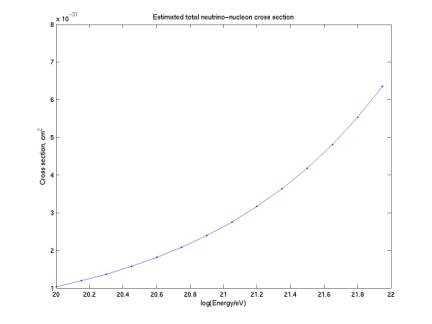
Figure 2
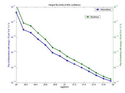
Figure 3
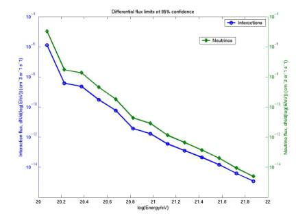
Figure 4
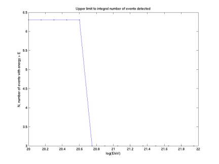
Figure 5
2/8/03
Limited bathymetry
allBathymetry.m
The
two figures below give rough bathymetry from the 62 phone coordinates that we
have. Depth contours are linearly
interpolated from hydrophone depths.
The
first figure gives literal depths (direct depths from the surface, not
ellipsoid heights, which are also availble).
The
second figure gives sea-floor heights normal to the SAUND plane, where the
SAUND plane is defined to be the least-squares plane fit to our 7 hydrophones
(inclined at 1 degree from the horizontal). In this figure it is apparent that the floor curves up around
our phones, cutting off our effective volume. However the data are insufficient to determine the entire
shape of our effective volume. It
would be best to have these data out to at least 10-20 km from our central
phone. It would also be best to have
sufficient resolution to determine if any hills in the sea floor are blocking
our effective volume.
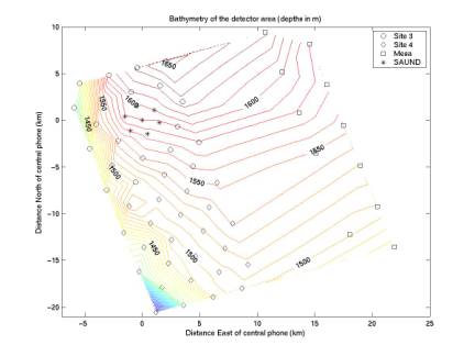
Figure 6
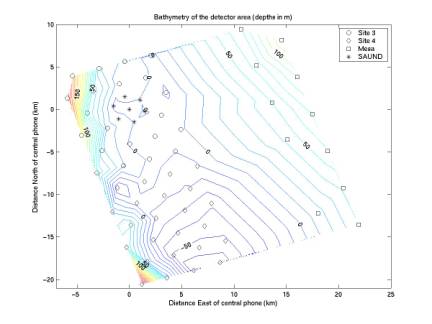
Figure 7
2/8/03
Limitations of our triangulation
variableT.m
variableC.m
Our
triangulation method (intersecting hyperboloids) assumes no error in phone coordinates,
signal times of arrival, or sound speed.
It also assumes spatially constant sound speed. The first plot shows the effect of
timing uncertainty on our depth determination. The depth is determined with various offsets (up to 1 ms,
quite a large offset) added to the first time of arrival. We see that the depth determination is
not sensitive to this uncertainty.
The
second plot shows the sound velocity profile (SVP) for the date of our light
bulb drop, July 30 2001. These
SVP’s should be available for many days from an FTP site but I’m
waiting to hear from an AUTEC employee about obtaining them.
We have been
assuming a sound speed of 1516 m/s, constant throughout depth and over seasons,
but our depth determination turns out to be quite sensitive to sound
speed. Assuming the second plot
(with sound speeds ranging from 1480 to 1550 m/s) is the appropriate curve for one of our candidate neutrinos,
we plot in the third figure the reconstructed depth as a function of a
particular (constant over depth) sound speed in this range. The depth uncertainty turns out to be
100 m. However we can iterate this
procedure again: we can focus on sound speeds that occur in this 100 m depth
range, a much narrower range of speeds (1491 to 1494 m/s). Applying this range of speeds gives a
range of depths of only 4 m.
This is a
particularly good case because the event is near the sea floor: for events near
the sea surface the entire SVP must be considered. But this is okay for us because we are primarily interested
in events near the floor.
If we have
SVP’s for many days throughout the year, hopefully we can apply this
method successfully and continue to use one effective speed for each
triangulation. It should be
possible to determine this from the reconstructed-depth profile once we obtain
the SVP’s. It would be much
more difficult to consider the sound speed varying over depth for each
triangulation, as the soultion would not be trivial and w have to calculate
hundreds of thousands of triangulations for our current data set.
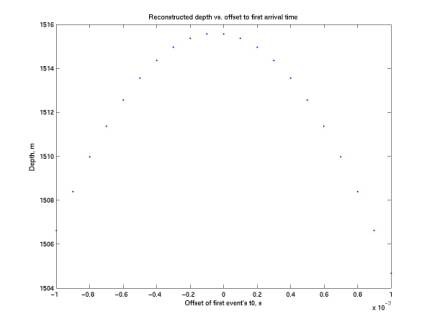
Figure 8
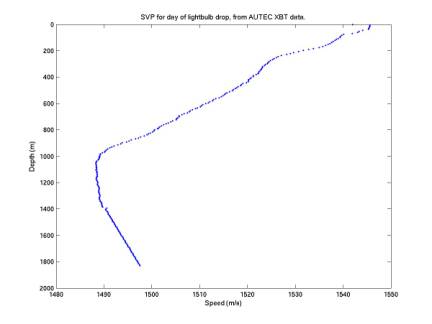
Figure 9
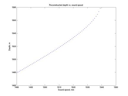
Figure 10
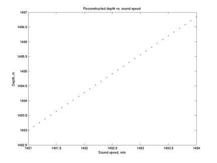
Figure 11