Log
14
Justin
Vandenbroucke
justinv@hep.stanford.edu
Stanford
University
3/20/03 –
This file contains log
entries summarizing the results of various small subprojects of the AUTEC
study. Each entry begins with a date,
a title, and the names of any relevant programs (Labview .vi files or Matlab .m
files – if an extension is not given, they are assumed to be .m files).
3/20/03
Ray tracing
rayTrace.m
I
have been neglecting ray refraction because earlier I determined it was
insignificant for a range of a couple km.
But if we want an effective volume stretching to 10 km, we need to check
ray paths at that range. With this
range, ray bending becomes significant.
In Figures 1-7, 10 rays are simulated at each of 7 depths. Rays are emitted at an angle below the
horizontal from 1 to 10 degrees, with a step size of 1 degree.
The
ray traces are rough estimates with an initial algorithm that will be
improved. When the rays begin to
curve back upward, they are cut short. The deeper the source is, the more the rays tend to bend back
upwards, limiting the horizontal range they can travel. This introduces a shadow: near the sea
floor our horizontal range is limited, with the range increasing with height
above the sea floor.
The
ray trace assumes the water is a layered medium, with sound speed varying only
in the z direction. According to
Gerald D’Spain at Scripps, horizontal sound speed gradients are typically
3 orders of magnitude below vertical gradients.
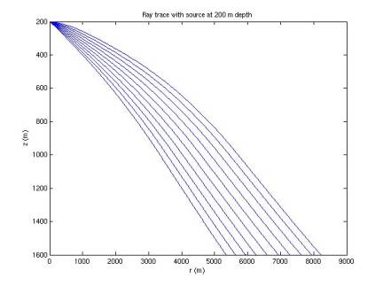
Figure 1
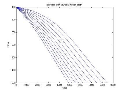
Figure 2
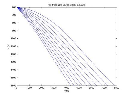
Figure 3
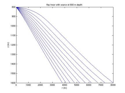
Figure 4
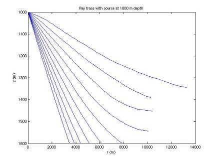
Figure 5
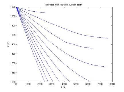
Figure 6
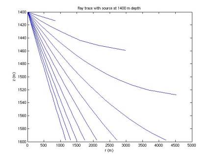
Figure 7
3/20/03
Refraction shadowing
calcShadow.m
plotShadow.m
So
ray tracing shows that refraction introduces a shadow, blocking events in some
parts of the water from being heard.
Unfortunately this shadow seems to correspond well with our effective
volume. Figure 8 shows the shadow
(blue curve). Only events above
the blue curve will be detected; rays from events to the right of the curve
will be refracted away from the detector. The red line gives the bounding curve for our effective
volume assuming no refraction, due to the shape of the radiation disk, for
2.4e22 eV (the volume ceases to grow near this energy). Our actual effective volume is then
bounded by the two curves.
However
it may be the case that the overall effects of refraction are to bend the
effective volume upward rather than blocking it. If we fully account for refraction, the red curve may be
bent upward. We need to simulate
the radiation disk including the effects of refraction to determine this (such
a simulation will depend on the orientation of the disk in the water). We may be able to do this simply by
considering a surface of the radiation pattern and bending each point on it
appropriately (ie we wouldn’t have to repeat the entire simulation).
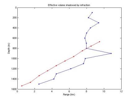
Figure 8
3/20/03
Improved ray trace algorithm
traceRay.m
rayTrace.m
plotRays.m
Following
conversation with Gerald D’Spain at Scripps, I devised an improved ray
trace algorithm that allows significantly better precision with a given CPU
time. The algorithm is explained
in Boyles, Allan: Acoustic Waveguides: Applications to Oceanic Science. It divides the water column into layers
and assumes that the sound speed is a linear function of depth within each layer. This is a much better approximation
than the previous one, which assumed the sound speed was constant in each
layer. Indeed, the AUTEC SVP is
well approximated by a 2-piece linear function, with the first piece linearly
decreasing with depth and the second part linearly increasing. This is the case in many ocean columns.
In
a medium with a constant-gradient sound speed, the ray paths can be shown to
follow the arc of a circle with radius determined by the mean sound speed and
the sound-speed gradient. The new
ray trace algorithm, traceRay.m, uses this feature in each layer. The layers can be chosen denser in
regions where the SVP is farther from linear. Arcs are calculated through each layer, but only the
endpoints are saved. Ray paths are
then drawn with each arc replaced by a straight segment, giving an allusion of
less accuracy than is actually achieved.
Figure 9 compares the old algorithm (blue) to the new one (green) for a
particular source depth.
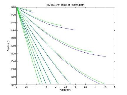
Figure 9
3/20/03
Direct determination of refraction shadowing
raysFromPhone.m
We
can determine the region shadowed by refraction directly by considering rays
emitted from a hydrophone. These rays are the same as those that
would be sent to the phone from a
source. In Figure 10, rays are
emitted from a phone at 1600 m depth at an angle above the horizontal from 1 to
30 degrees, every 1 degree (blue).
Rays are also emitted at an angle of 10-1 through 10-10
(every factor of 10) degrees to show the asymptotic boundary of the shadow
region (red).
Rays
are terminated when they reach the horizontal and begin to turn around (beyond
this point they follow the reflection of their first path. We can compare the shadow region in
Figure 10 (all white space to the right of the traces) with the indirect
determination in Figure 8 (blue curve).
In
general, if a ray is emitted horizontally, it will travel toward the sound
speed minimum (at 1100 m in our case) and then turn around where the sound
speed increases again to the value where the ray originated. The ray continues to oscillate between
these two turning points.
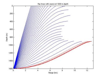
Figure 10
3/25/03
Full ray trace compared to
straight paths
plotRays.m
I
extended the ray tracing algorithm to continue tracing the rays when they
reverse vertical direction. In
Figures 11-17, red rays represent those determined by ray tracing; black rays
represent the case of zero refraction.
Recall the sound speed minimum is at ~1100 m. Rays are terminated when they hit 0 depth, 1800 m depth, or
a total path length of 10 km.
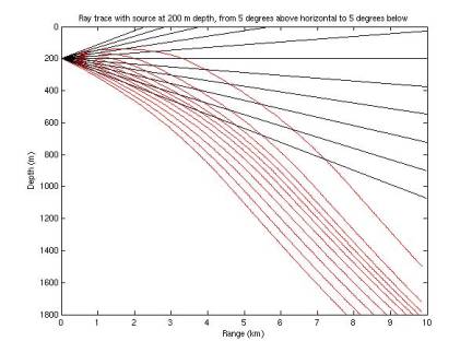
Figure 11
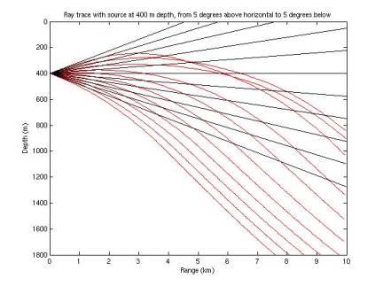
Figure 12
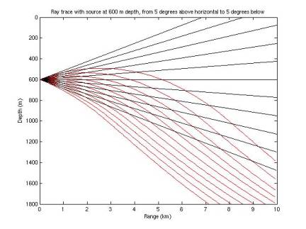
Figure 13
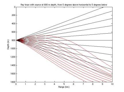
Figure 14
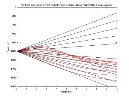
Figure 15
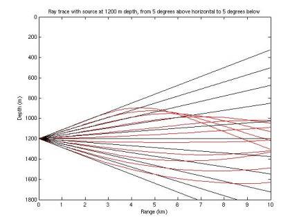
Figure 16
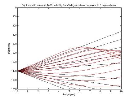
Figure 17
3/25/03
Effect of refraction on acoustic radiation disk
plotDiskVertices.m
Refraction
affects the acoustic rays from a neutrino shower, bending the equal-amplitude
surface enveloping the radiation pattern.
We can determine the correct radiation pattern by starting with an
unbent disk and bending a sample of rays that terminate on the disk. This is done for horizontal disks
(vertical neutrino incidence) in Figues 18-22 for various interaction depths
(200, 800, 1000, 1400, and 1600 m).
In each plot the original and bent disks are drawn, as are the 7
hydrophones. A black curve
connects neighboring ray endpoints to sketch the envelope of the radiation
pattern.
Above
the sound speed minimum (at 1100 m), the disk is bent downward; below it the
disk is bent upward. At depths
near and below the sound speed minimum, there are some special rays that leave
the group. The flux of these is
low, however, indicating the amplitude is correspondingly decreased.
Figure
23 shows an example of a refracted disk that actually contains multiple hydrophones. The neutrino interaction is at depth
1590 m and zenith 1 degree.
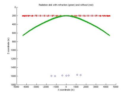
Figure 18
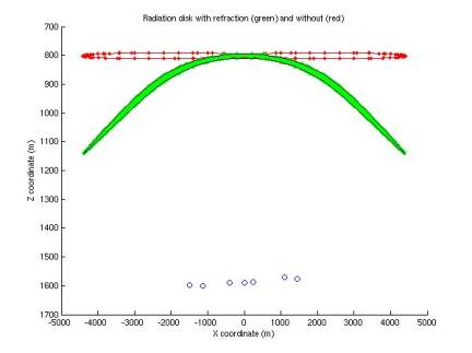
Figure 19

Figure 20
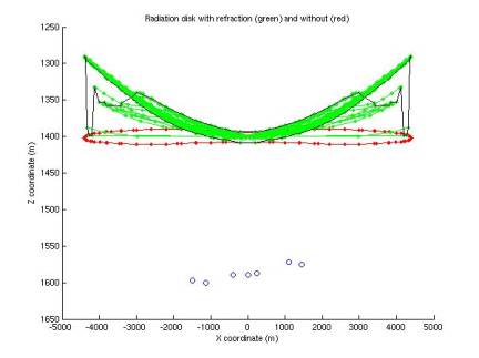
Figure 21
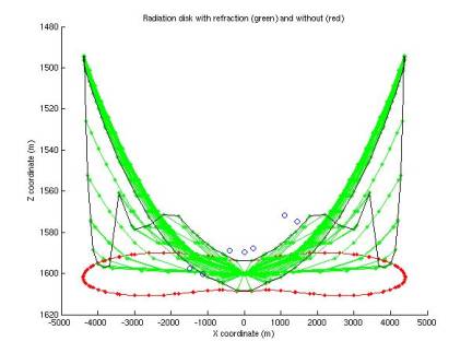
Figure 22
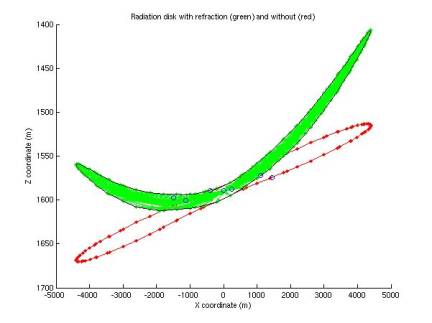
Figure 23