Log
15
Justin
Vandenbroucke
justinv@hep.stanford.edu
Stanford
University
3/28/03 –
This file contains log
entries summarizing the results of various small subprojects of the AUTEC
study. Each entry begins with a
date, a title, and the names of any relevant programs (Labview .vi files or
Matlab .m files – if an extension is not given, they are assumed to be .m
files).
3/28/03
Ray trace bug fixed
traceRaySetLength.m
The
bent radiation had some rays (those near the horizontal) that diverged from the
others, as shown in Figure 1. This
caused the envelope of the radiation disk (black line, connecting successive
ray endpoints) to have a strange shape.
This
was due to a bug in determining the ray turning points. I was interpolating depth as a function
of sound speed, but this function is double-valued from 900 m to 1800 m. Choosing the appropriate branch before
interpolating fixed the ray tracing (Figure 2).
Both
unbent (red) and bent (green) rays are plotted on the right and left sides from
only 1 degree above the horizontal to 1 degree below, every 0.02 degrees. The disk is well determined by this
small range, meaning it only spans ~2 degrees.
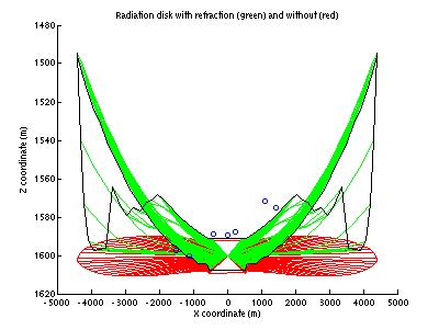
Figure 1
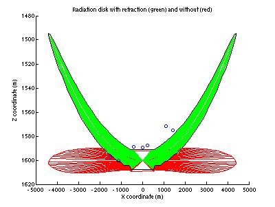
Figure 2
4/2/03
Calculation of
acceptance without
refraction
calcAcceptanceMC.m
plotAcceptance.m
calcAcceptanceVsE0.m
plotAcceptanceVsE0.m
plotDiskVertices.m
The
detector acceptance must be recalculated now that we realize refraction is a
significant effect. As shown
above, the radiation disk curves on the same distance scale as the detector, meaning
that a radiation disk of radius 10 km that is 7 km away from the array,
coplanar with the array, will not necessarily trigger the phones (it may curve
away before reaching the phones).
The
acceptance calculation accounting for refraction is significantly more involved
than when we neglected refraction.
From Nikolai’s simulation of the signal at arbitrary receiver
positions relative to the neutrino, we have the envelope of the radiation disk
for a given neutrino energy and filter-value threshold.
This
disk is defined by a set of O(100) vertices in 2D, such as that in Figure
3. The disk is a surface of
revolution about the vertical axis of the figure. The vertices are symmetric about the y axis. For points with nonzero x, each pair of
vertices with equal y coordinates determines a circle, about the y axis, of the
radiation disk surface. The
surface is thus defined by a set of circles.
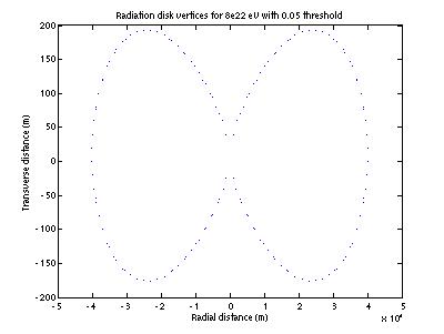
Figure 3
In
general, to calculate acceptance at a particular neutrino energy we choose
random neutrino shower coordinates (x, y, z, theta, phi). We then count the number of phones that lie within the radiation disk,
as defined by the set of circles.
We do this phone-by-phone, determining one-by-one whether each phone is
inside the disk.
In
the case of no refraction, the ocean is isotropic and rather than having to
rotate the radiation disk to (phi, theta) we can equivalently leave the disk
fixed and rotate the phone appropriately.
This is conceptually and computationally much easier.
We
really only care about the axis between the neutrino interaction point
(idealized to a point at the center of the radiation pattern) and the
phone. The question is on which
side of the phone the disk cuts through this axis. We determine this by choosing any plane containing the axis.
We
choose the plane that is perpendicular to the radiation disk. With this choice, the intersection of
the plane and the disk is simply the 2D set of vertices shown in Figure 3. So we need not manipulate these vertices
at all and can simply rotate each phone appropriately relative to them, then
determine whether the phone lies within the closed curve determined by the
vertices.
4/2/03
Calculation of
acceptance with refraction
calcAcceptanceRayTrace.m
plotAcceptanceRayTrace.m
calcAcceptanceRT.m
With
refraction, the ocean is not isotropic and we must actually rotate the whole
disk, leaving each phone fixed.
Again we do this phone-by-phone.
In this case each circle of the radiation disk is bent by
refraction. Each ray bends
vertically and lies in a vertical plane.
So instead of choosing the plane that cuts the disk perpendicularly, we
choose the plane (through the phone – interaction point axis) that is
vertical. This plane generally
cuts the disk obliquely, not perpendicularly. So we must first determine the vertices of this oblique
cross section. We can then bend
the rays within this plane, because it was chosen to be vertical.
To
determine the oblique cross section, we transform each vertex of the original
(perpendicular) cross section.
Consider each pair of vertices that determine a circle of the radiation
disk. These two vertices are
transformed by determining the intersection of the circle with the vertical
plane.
Once
we’ve determined this cross section, we bend each ray ending on a vertex
to determine the oblique cross section of the refracted disk. We can then determine whether the phone
lies inside or outside this set of vertices, as before.
Note
that the determination of the original cross section through the radiation
pattern, and the bending of rays, must be done separately for each phone. Due to the many rays that have to be
traced (~ 100 per phone, so ~700 per neutrino interaction), counting hit phones
with refraction takes O(100) times as long as without refraction.
This
strategy was implemented but was exceedingly slow, so slow that it took
multiple CPU-days to get the Monte Carlo integration to converge. Only after implementing this method and
realizing that it was too slow did I realize there was a simpler method.
4/7/03
Calculation of
acceptance with refraction in 1D instead of 2D
findRay.m
traceRaySetDepth.m
plotDiskVerticesPolar.m
calcAcceptance1RayTrace.m
The
method described above requires, for each phone, sampling rays in a vertical
plane to determine a 2D cross section of the radiation disk, then determining
whether the phone lies inside the cross section.
A
simpler method involves determining, for each phone, the single ray from neutrino interaction to phone. We then only need to determine whether
the ray reaches the phone in a short enough path length that it is still within
the radiation pattern.
The
first step of this method is determining a ray between two arbitrary points,
the source and the receiver. This
is implemented in findRay.m. This
is unfortunately not a direct calculation but involves an iterative
solution. Direct calculations can
be made to trace a ray emitted from an arbitrary point at an arbitrary angle,
but it is not generally known a priori which angle the ray should be emitted at to reach the receiver
position.
The
general ray trace problem (from an arbitrary point at an arbitrary angle) only
has two inputs: source depth and initial angle (we assume the sound speed does
not vary horizontally). So to
solve the source-receiver problem we trace multiple rays with multiple initial
angles, from the source depth to the receiver depth. The range (horizontal distance traveled) is determined for
each of these rays. The ray we
seek is that ray with a range equal to the horizontal distance between the
source and receiver. We implement
this with a least-squares algorithm, seeking the initial angle that minimizes
the difference between the desired range and the ray range squared.
findRay.m
determines the initial angle and the path length of the single ray from source
to receiver. The next step of this
method, once we have the ray length and angle, is to compare it to the
radiation pattern. The ray
represents the path of an arbitrary sound (not necessarily a neutrino) of
arbitrary amplitude. We must
determine whether this path is short enough to lie within the neutrino
radiation pattern at the emitted angle.
We do this by using a lookup table for the disk vertices (as shown in
Figure 3) in polar coordinates. An
example of this (for the same energy as Figure 3) is shown in Figure 4.
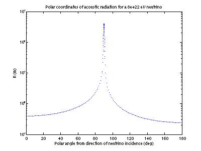
Figure 4
All
of the vertices necessary to represent a disk in rectangular coordinates (such
as that in Figure 3) are contained within ~1 degree. That is, the radiation lobe is confined to a width of 1
degree. This means that direct
conversion of the vertices in Figure 3 to polar coordinates is inadequate. The vertices in the rectangular plot
had to be supplemented before conversion to polar coordinates, in order to
determine the behavior of R(theta)
at the other 179 degrees. This was
done by assuming the radiation disk crosses the y axis perpendicularly. If this is the case, R(theta) is as follows
h1/cos(theta), 0
< theta < pi/2
h2/cos(pi-theta), pi/2
< theta < pi,
where h1 is the vertical distance of the first y intercept
above the origin, and h2 is the
distance of the second y intercept below the origin. These values were used for theta at every integral degree
from 0 to 89 and 91 to 180.
The
behavior of R(theta) in this
interpolated region is important, and we should verify the assumption that the
radiation crosses the axis perpendicularly and we can interpolate it from the
nearest vertex to the axis.
From
the azimuth and zenith of the neutrino, and the initial angle of the
neutrino-receiver ray, it is straightforward to determine the initial angle
between the ray and the direction of incidence. This angle is exactly theta in our radiation pattern plot (Figure 4). The geometry involved in determining theta is much simpler than what was necessary for the
planar method. Once we know theta
and the ray path length (s), we
simply look up R(theta) for the
appropriate neutrino energy. If s
< R, the ray reaches the receiver
while still inside the radiation envelope, and the neutrino is detected by the
receiver.
This
method assumes that the acoustic signal depends only on the initial ray angle
and total path length, not on the amount of refraction. That is, we assume the signal is
neither scaled nor distorted by refraction, as it might be.
4/7/03
Comparison of run times
Roughly
1e5 Monte Carlo points (independent random choices of neutrino x, y, z, theta,
phi) are necessary for convergence of the acceptance calculation. We have calculated acceptance with
three algorithms:
1) Assume no refraction; rotate phones with fixed 2D
rectangular disk coordinates
2) Assume refraction; rotate 2D rectangular disk
coordinates with fixed phones
3) Assume refraction; determine the single ray from
neutrino to each phone
Table 1 gives a comparison
of run speed and total run time necessary for the three algorithms (on a single
CPU). Algorithm 3 is the best
so far considering both accuracy (accounting for refraction) and speed.
Table 1
4/8/03
Results of acceptance
calculation
calcAcceptance1RayTrace.m
plotAcceptanceRayTrace.m
The
algorithm described above (calcAcceptance1RayTrace.m) was run for energies 2e21, 4e21, 8e21, 2e22, 4e22,
and 8e22 eV. Distributions rae
given below for the highest energies.
105 Monte Carlo points (x, y, z, theta, phi) were generated,
and the number of phones hit by each event were counted. Figure 1 gives the distribution of the
number of phones hit.
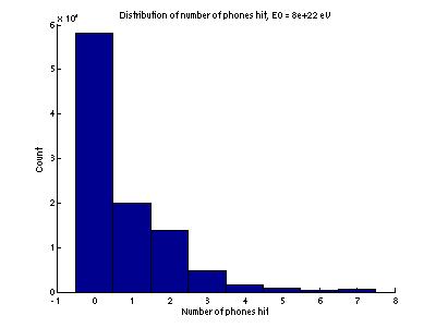
Figure 5
Figure
2 gives a side view of the distribution of 4-phone events. We are using an SVP from the day of the
light bulb drop. This SVP extends
to 1800 m depth. We have generated
points from 1400 m to 1800 m (even though the sea floor is at 1600 m; we ignore
it for this step). It is unclear
why there is an excess of points in the plane of the phones. We might expect such an excess not
exactly in the flat plane but bent upward by refraction. The red curve represents a typical
refracted ray in this region. It
was emitted horizontally from 1600 m depth.
The
next step is to appropriately account for the sea floor. The events plotted in Figure 6
represent those detectable by a detector at the same depth as the SAUND
detector, but with the sea floor 200 m lower than it actually is. Events below the red curve will
typically hit the sea floor and will not actually be detected. Properly accounting for the sea floor
will remove roughly those events below the red curve. It appears this will reduce our acceptance by a couple
orders of magnitude.
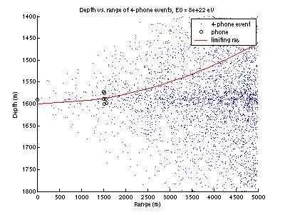
Figure 6
Figure
7 gives the distribution of path lengths of (refracted) rays between each Monte
Carlo event and the central phone.
It is cut off at 5 km, the radius at which we have chosen to cut off our
effective volume. Beyond this
distance two effects make event reconstruction difficult; (1) refraction
becomes an even stronger effect and (2) points that are not very close may have
similar time differences of arrival (position reconstruction uncertainty
increases with range). The first
effect is independent of the detector spacing; the second is determined by
detector spacing.
Figure
8 gives the same distribution, but only for those events that trigger 4 phones
rather than for all events generated.

Figure 7
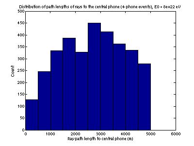
Figure 8
Figure
9 gives a top view of those events that trigger 4 phones or more.
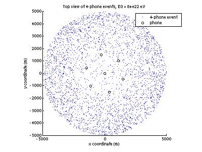
Figure 9
Figure
10 gives the distribution of neutrino zenith for 4-phone events. Figure 11 gives the same distribution
for all generated events. They are
generated isotropically, but only those near vertical are detected.
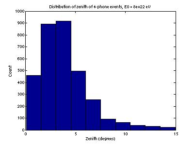
Figure 10
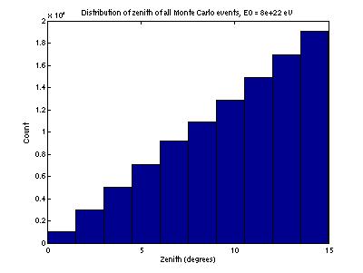
Figure 11
Figure
12 shows zenith vs. range of detectable events. As the range increases, the maximum detectable zenith
increases.
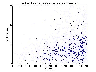
Figure 12
Figure
13 gives the distribution of neutrino azimuth. Detection appears to be independent of azimuth.
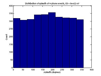
Figure 13
Figure
14 gives the distribution of depths of detected neutrinos. The limits used for both zenith and
depth in the Monte Carlo integration were not quite large enough and will be
extended.
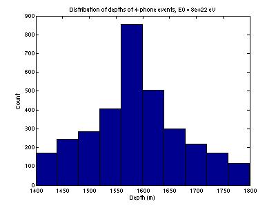
Figure 14
4/8/03
New acceptance curve
calcAcceptanceRT.m
plotAcceptanceVsE0.m
Figure
15 presents the new acceptance curve in addition to previous ones. The top three curves represent those
calculated neglecting refraction.
The top one assumes infinite homogeneous water; the middle one limits
our effective volume at 10 km; the third limits it at 5 km. The bottom curve includes refraction
and limits the effective volume at 5 km.
It is lower than the initial curve by 3 orders of magnitude at high
energy, but is actually higher by one order of magnitude at low energy. I’m not sure why this is; perhaps
the curvature induced by refraction is somehow beneficial at lower energy.
The
curve will lower even further when we include the shadow effect of the sea
floor.
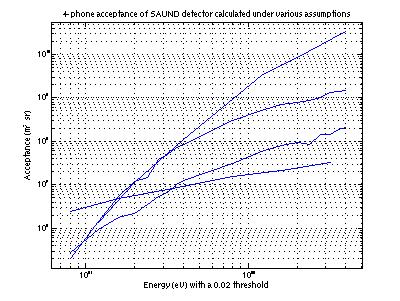
Figure 15