Log 16

Justin Vandenbroucke

justinv@hep.stanford.edu

Stanford University

4/13/03–

This file contains log entries summarizing the results of various small subprojects of the AUTEC study. Each entry begins with a date, a title, and the names of any relevant programs (Labview .vi files or Matlab .m files – if an extension is not given, they are assumed to be .m files).

Note: Higher-resolution versions of the figures are available. If a log has URL dirname/logLL.html, Figure FF of the log should be at URL dirname/FF.jpg.

4/13/03

Caustics

calcAcceptance1RayTrace.m

[to be added]

5/2/03

Precise, fast localization achieved

reconInterp.m

plotReconInterp.m

I finally figured out a scheme for 3D localization that that achieves high-precision localization quickly. For two weeks I’ve been trying variations on a lookup table of TDOA’s. From a 3D grid of points I trace rays to each phone, calculating travel time to each phone. I can then determine a lookup table of TDOA’s, and TDOA’s of actual events can be compared to this lookup table. The best point is chosen from the lookup table with a least-squares metric between the measured and lookup-table TDOA.

Generating the lookup table for a particular SVP with 100 m spacing in all 3 directions, spanning a cylinder of radius 5 km about the central phone, takes 3 hours on 6 CPUs. However this resolution is not sufficient; the nearest point is not chosen. Even if it was, our resolution would be at best O(100) m, but it is actually several hundred m with this method. Increasing the resolution to 50 m takes 2³ = 8 times longer to generate the table, or 24 hours. But the resolution is not much better.

I also tried doing a least-squares minimization with the best grid point only as an initial guess. I allowed the optimization to range in 3D, and traced rays at each test point to determine TDOA’s. Requiring the optimization to terminate in O(30) s, this did not achieve much better precision than staying on the grid.

But the each TDOA is a fairly smooth 3D field. So it can be interpolated linearly between grid points, without having to start over again with a ray trace. The interpolation takes multiple orders of magnitude less time for each point. It achieves very good precision, O(1) m, with very little time, 3 s per localization for a 1.5 km cylinder of grid points or 20 s per localization for a 5 km cylinder . The grid points have a resolution of 100 m.

Our resolution varies over the 3D volume of detector. It is worst near the sea floor and at large radii outside the peripheral phones. Here we examine the resolution as a function of horizontal location. We bin the points in 1 km by 1km squares by actual Monte Carlo event location, and consider the horizontal and vertical reconstruction precision of points in each bin. We can then draw contours representing the variations in resolution over the horizontal extent of the detector.

Note that the precision discusses here is only the precision of the minimization convergence, assuming no measurement error. The next step will be to add measurement error in the SVP, hydrophone locations, and event times of arrival. Preliminary estimates indicate that even with these errors, 10 m resolution will be possible in the bulk of the detector, with 100-200 m resolution at the worst locations (at 1400-1600 m depth and 3-5 km radius).

Figure 1 shows mean horizontal error. It is typically less than 1 m within the array and 10 m within 5 km. Figure 2 shows mean vertical error. It is typically less than 10 m inside the array (where means are consistently 1-2 m, but they do not vary smoothly over space, so no contour is supported below 1 m) and 30 m within 5 km.

These points are all Monte Carlo, with ~16,000 points total divided among ~75 horizontal bins, giving ~200 points per bin.

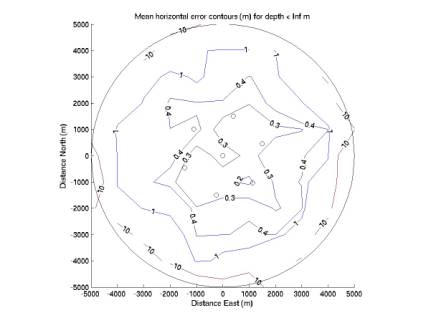
Figure 1

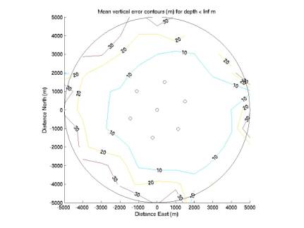
Figure 2

We should consider maximum errors in addition to mean errors. In each horizontal square bin, we can compute the maximum horizontal and vertical errors among the ~200 points. The resulting contours are given in Figure 3-8. Figures 3-6 give contours for vertical error. Figure 3 only considers points with depth below 800 m, Figure 4 below 1200 m, and Figure 5 all points. In the top half of the depths, vertical error is very low. It increases steadily below 800 m, with the highest values at the sea floor.

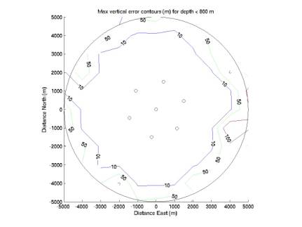
Figure 3

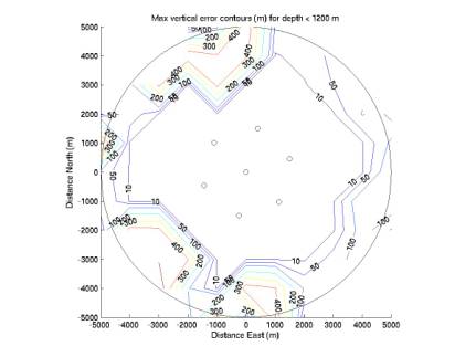
Figure 4

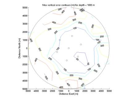
Figure 5

Figures 6-8 give corresponding contours for horizontal error. Horizontal error does not vary with depth as vertical error does, but remains quite good throughout the volume.

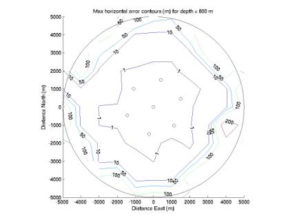
Figure 6

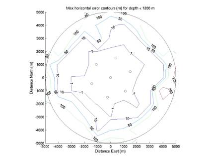
Figure 7

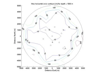
Figure 8

By plotting the maximum errors we can look for extreme outliers. It’s good that the error distributions are well-behaved. They are quite small within the array and are reasonable far outside the array.

We can also divide the data into horizontal slices and consider the max and mean errors in each layer. Figures 9 and 10 show the mean error profiles. Figures 11 and 12 show the max error profiles. Slices are 100 m thick.

Note in Figure 12 the two segments at deep depths that appear to be reversed. Apparently there is some symmetry in the TDOA metric about 1400 m, so 1600 m events are reconstructed at 1200 m and vice versa. It may be that the algorithm finds a local minimum. If the two minima are at similar values of the metric, it will be impossible to distinguish between them. However I believe this only happens far outside the array.

In general the reconstruction is quite good within 1-2 km radius, where I expect most of our events are. Our reconstruction is bad only where we do not expect many events. So I expect we will have precise reconstruction for most background events, allowing us to reject them based on region of the detector.

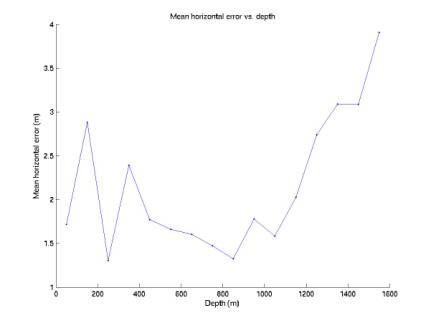
Figure 9

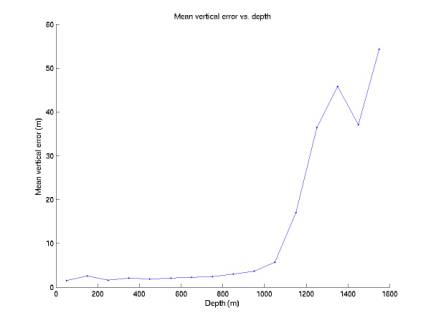
Figure 10

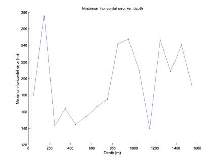
Figure 11

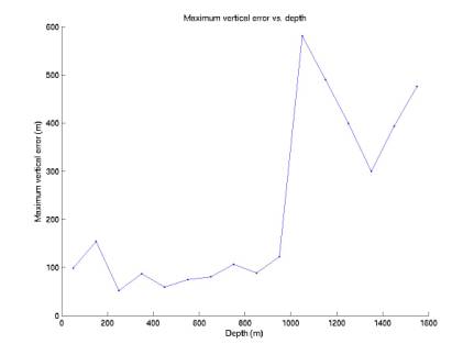
Figure 12