Log 17
Justin
Vandenbroucke
justinv@hep.stanford.edu
Stanford
University
5/5/03–
This file contains log entries summarizing the results of various small subprojects of the AUTEC study. Each entry begins with a date, a title, and the names of any relevant programs (Labview .vi files or Matlab .m files – if an extension is not given, they are assumed to be .m files).
Note: Higher-resolution
versions of the figures are available.
If a log has URL dirname/logLL.html, Figure FF of the log should be at
URL dirname/FF.jpg.
5/5/03
Direct error estimates
plotUncertainty.m
We
can get a good handle on the localization precision we expect with some simple analytical
considerations. Event locations
are determined by minimizing a least-squares metric. We assuming 4 nearest neighbors (forming a diamond) are hit. This means in particular that the 7th
(central) phone is hit. The events
are detected at times ti, i=1,2,3,7. The
four times of arrival determine three measured time-differences of arrival, Tmi,
i=1,2,3 (the m is for measured). We compare these to
theoretical time-differences of arrival, Ti(r), i=1,2,3. Ti depends on the position of the source in 3D, r (as well as which SVP and hydrophone positions are
being used). We sample Ti with a lattice.
We then have a finite set of Ti to be compared with our single Tmi. We find
the closest Ti to Tmi by minimizing a metric, m = sum[(Ti-Tmi)2,
i=1,2,3]. With sufficient lattice spacing, the lattice Tmi point that minimizes the metric is a good first guess
for the location of the event. We
can then interpolate Ti
for points off the lattice, and minimize m within a neighborhood of our first guess.
If
we achieve zero position uncertainty, m=0. In reality we have three
sources of measurement error: SVP, timing, and hydrophone location. Uncertainty in each of these introduces
uncertainty in our measured TDOA.
The range of TDOA values within our uncertainty then determine a range
of metrics above zero. We are not
able to resolve the location to a single point at which m = 0, but to a region or regions of points for which m
< mmax. mmax is determined by our various measurement
uncertainties.
Now
recall that a ~1500 m/s sound speed determines equivalence between 1 ms and 1.5
m. This is the basis for comparing
distance and time uncertainties. 1
ms is the size of our entire captured waveform. The actual impulsive signal typically spans less than this
duration, and it has some maximum/central cycle that is only ~0.1 ms wide. So we expect our timing uncertainty to
be below 1 ms. 1.5 ms, on the
other hand, is a small distance compared to the scale of the detector. The hydrophone location uncertainty is
probably ~5 m. This uncertainty
dominates the timing uncertainty.
Similarly, SVP’s vary up to ~ 5 m/s from month to month. So for a sound travel time of O(1) s,
we expect SVP uncertainty to contribute similarly to hydrophone location
uncertainty. We expect the
distance scale of these two effects, 5 m, to determine our localization
precision. A deviation of 5 m (3
ms) shifts our metric by ~3*(3 ms)2 = 3e-5 s2. So we can only resolve the event
location to the region(s) with m < ~3e-5.
We
can get a feel for our practical uncertainty by looking directly at deviations
in path length. According to the
above considerations, we can only resolve sources that have source-receiver
path lengths that differ by O(5).
We can use this fact to estimate upper bounds of our vertical and
horizontal uncertainty.
Consider two points a horizontal distance R from a single phone. The path lengths to the phone (we assume they are not
refracted – refraction does not significantly affect times of arrival,
and affects TDOA’s even less) are S1 and S2.
First
we consider vertical uncertainty.
There is some maximum vertical distance we can separate the two points
before their path lengths differ by more than 5 m. This distance depends on R and on the depth. This distance is our vertical
resolution. Figure 13 shows this
resolution vs. depth for various values of R. Dashed lines are for 10 m path-length resolution; solid are
for 5 m. We see that vertical
resolution is best near the sea surface and horizontally close to the hydrophone. At 1 km distance the resolution is
better than 100 m for all but the bottom 100 m. At 10 km distance the resolution is better than 100 m for
roughly the upper half of the sea column.
Events at the edge of our 5 km – radius detection volume will have
R = 3.5 to 5 km.
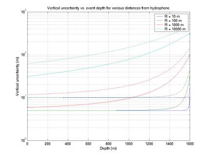
Figure 1
Figure
14 is the equivalent plot for
horizontal uncertainty. Horizontal
resolution is complementary to vertical resolution: worst near the surface and
directly above the phone. However
this picture is much worse than will actually occur when 4 phones are
used. In that case, even if an
event is directly over one phone, it will be ~1 km from others
horizontally. The minimum horizontal
distance from any phone is a few hundred m. So we expect horizontal resolution of at worst a few
10’s of m throughout the detector volume.
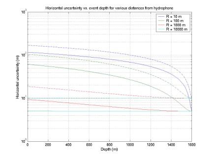
Figure 2
5/12/03
Location reconstruction
algorithm applied to data
PlotLocalizeCandidates.m
Our localization algorithm has been applied to actual data. There are about 8e5 4-phone combinations to try. It would be great to reduce this to
90,000
points
Figure 3
Figure 4
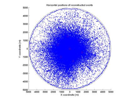
Figure 5
Figure 6
Figure 7
Figure 8
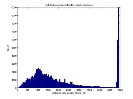
Figure 9
5/12/03
Localization applied to
random times uniformly distributed and in coincidence
plotRandomTimesOnGrid.m
30,000 points: in coincidence
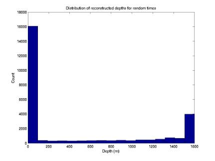
Figure 10
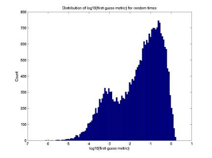
Figure 11
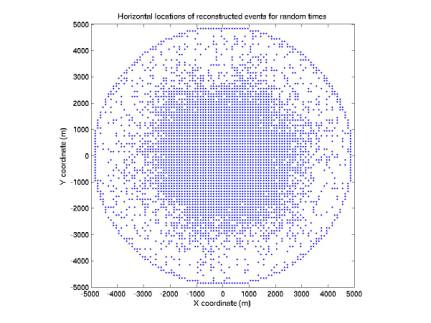
Figure 12
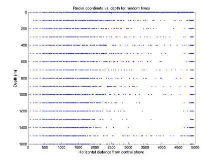
Figure 13
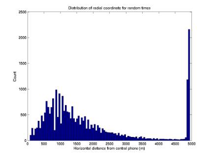
Figure 14
5/12/03
Localization applied to random
times uniformly distributed but not in coincidence
plotRandomTimesOnGrid.m
50,000 points: not in
coincidence
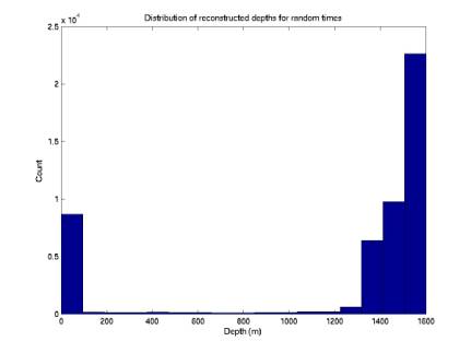
Figure 15
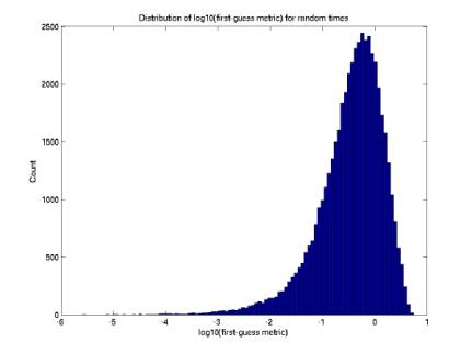
Figure 16
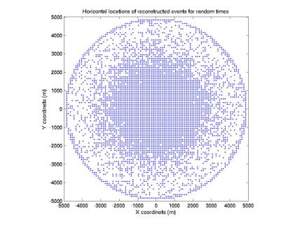
Figure 17
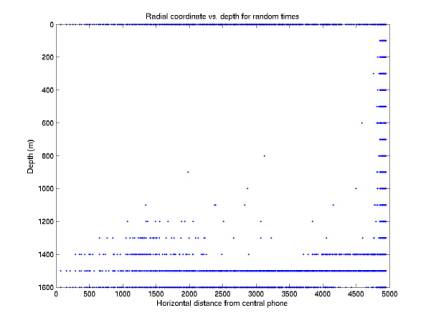
Figure 18
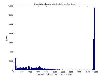
Figure 19
Distribution of num combos / hour