Log 18
Justin
Vandenbroucke
justinv@hep.stanford.edu
Stanford
University
5/15/03–
This file contains log entries summarizing the results of various small subprojects of the AUTEC study. Each entry begins with a date, a title, and the names of any relevant programs (Labview .vi files or Matlab .m files – if an extension is not given, they are assumed to be .m files).
Note: Higher-resolution
versions of the figures are available.
If a log has URL dirname/logLL.html, Figure FF of the log should be at
URL dirname/FF.jpg.
5/15/03
Rate of 4-phone candidates
numLocalizationCandidates.m
Figure
1 gives the number of localization candidates (sets of 4 events at neighboring
phones in coincidence) per hour over time. Figure 2 gives the cumulative number of candidates over
time. Note that this data rate
spans 6 orders of magnitude! It is
very important for us to try to stabilize this data rate as much as
possible. We have 6e5 candidates
in 168 days of integrated live-time.
This means our mean is only 150 candidates per hour (one every 24 s), but
one hour has 1e5 candidates!
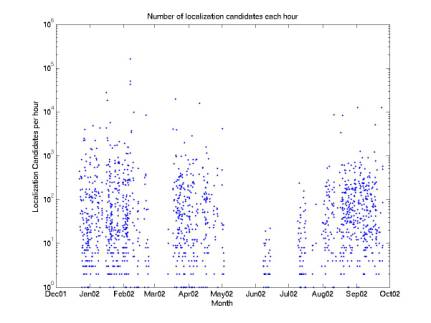
Figure1
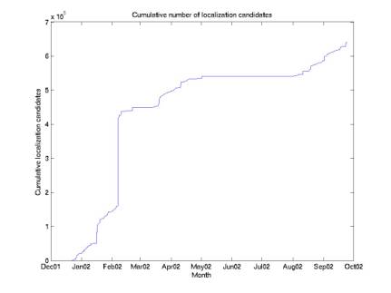
Figure 2
5/15/03
Rate of events during
quiet times
plotQuietCandidates.m
We
determined earlier that data acquired with threshold less than or equal to
0.024 account for ~90% of our integrated exposure (they dominate because the acceptance is much greater for them). So we
can neglect the minutes of data taken with threshold above this value and focus
only on these “quiet” minutes. Figures 1 and 2 give the data rate
considering only quiet candidates.
This reduces the total number from 6e5 to 6e4.
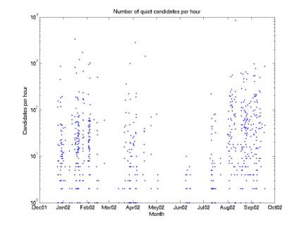
Figure 3
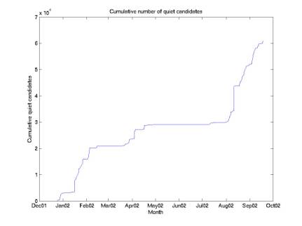
Figure 4
5/16/03
Side view of
reconstruction error
sideResolution.m
Figures 1 and 2 give side views of the contours of localization error, for vertical and horizontal error. The contours give maximum errors among ~90,000 Monte Carlo points. The points are chosen uniformly in a cylindrical volume (not uniformly in the side view). These are consistent with figures in Log 16.
The vertical error shows two trends. Above 1300 m: it is generally best for low depths and radial coordinates and worst for large depths and large radial coordinates. Below 1300 m: it is strongly limited by the curvature of the hydrophones. Because the array is flat, moving the source vertically within this range does not change travel times significantly.
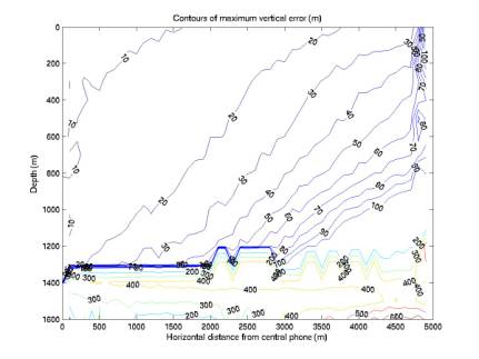
Figure 5
Horizontal
reconstruction is quite good throughout all depths, out to the boundary of the
lookup table (presumably this is just because it is at the boundary).
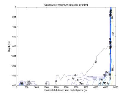
Figure 6
5/16/03
Event rates and combinatorics
candsPerMinute.m
plotCandsPerMinute.m
Figures
7-10 apply only to quiet data, the data taken during minutes with threshold <=
0.024.
Event
rates are quite unstable, both for single-phone triggers and 4-phone
combinations of triggers (“combinations” or “candidates”). Figure 1 is a histogram of the number
of combinations per minute, on a log
scale. We see 100 combinations per
minute is typical, but some minutes have as many as ~30,000. We should certainly stabilize this
online in SAUND-II. We may also be
able to stabilize it offline for the current data set. It may help us achieve some data
reduction.
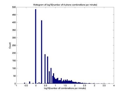
Figure 7
Figure
8 gives the same histogram spread out over time.
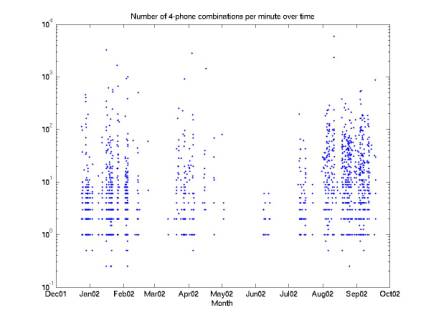
Figure 8
Figure
9 gives increasing number of combinations per minute on the horizontal axis,
and the cumulative sum of combinations on the vertical. It shows that the total number of
combinations (during quiet minutes) is 6e4. If we neglect minutes that are swamped, e.g. with >100
combinations per minute, we can reduce this to 2e4. If we neglect minutes with >100 combinations per minute,
we can reduce it to 5e3.
We
can imagine raising the threshold offline until there are 10-100 combinations
per minute or fewer. We have to be
careful that we do this legitimately though, particularly because we are
applying it directly to each minute (rather than setting it before a minute
occurs, as is done online). We
need to make sure we don’t always raise the threshold when there are
events, particularly that we wouldn’t raise the threshold when a neutrino
occurs.
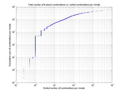
Figure 9
Above we have considered only 4-phone combinations. Sometimes we have a minute with 50 single-phone triggers that all occur within 1 second, resulting in 10,000 4-phone combinations. In Figure 10 we give statistics for the single-phone triggers composing 4-phone combinations. Although there are 6e4 combinations, there are only 2e4 triggers, or 2e4/4 = 5e3 possible physical acoustic events.
If we re-threshold offline we would aim to pick out these 5,000 physical events. Note that we already know we have at most 5,000 4-phone acoustic events, we just don’t know which ones they are.
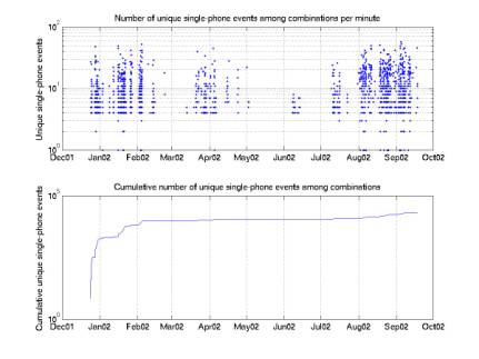
Figure 10
5/16/03
Combinatorics for an example
minute
combosOneMinute.m
Here’s
an analysis of a minute with very many 4-phone combinations (in fact the most
for one minute, over 1,000).
Figure 1 gives event number vs. time stamp.
The
problem is that there are only ~50 events, a good number considering our target
of 60, but they all occur within a window of 0.6 s! This means that the coincidence window does nothing and all
4-phone combinations must be considered.
There are combinations among all 6 4-phone diamonds. Consider diamond 3, for example (phones
2, 3, 4, and 7). At these phones,
there are 7, 11, 12, and 1 event respectively. This means there are a total of 7*11*12*1 = 924 combinations
just for diamond 3!
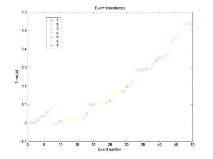
Figure 11
Figure
12 shows the trigger value of the events.
The online threshold was 0.020.
Raising it offline one notch, to 0.024, would eliminate the single
central-phone (phone 7) event and would hence eliminate all combinations.
This
is a very extreme example, but such offline rethresholding based on
combinatorics would probably be helpful overall. Note also that the real root of the problem is that we had
poor data quality to begin with.
Hopefully the next generation will address these problems.
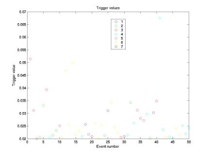
Figure 12
5/16/03
Strategy for candidate reduction
Here
is an optimistic strategy for reducing the number of neutrino candidates:
600,000 ->
60,000 restricting
to quiet minutes
60,000
-> 6,000 localization
6,000 -> 600 offline
re-thresholding to reduce combinatorics
600 -> 60 waveform
matching; Nikolai parameters
60 ->
6 examining
events by eye