Log 19

Justin Vandenbroucke

justinv@hep.stanford.edu

Stanford University

5/23/03

This file contains log entries summarizing the results of various small subprojects of the AUTEC study. Each entry begins with a date, a title, and the names of any relevant programs (Labview .vi files or Matlab .m files – if an extension is not given, they are assumed to be .m files).

Note: Higher-resolution versions of the figures are available. If a log has URL dirname/logLL.html, Figure FF of the log should be at URL dirname/FF.jpg.

5/23/03

Corrected acceptance calculation

genMC.m (directory mat_files/genMCExtended/ on erinyes)

goodPoints.m

plotGoodPoints.m

Acceptance was recalculated with Monte Carlo data points. 10⁵ points were chosen uniformly in volume and source direction for each of 6 neutrino energies. For each point, rays were traced to each of the 7 hydrophones. The path length to the phone and the angle of the ray as it left the interaction point were used to determine whether the ray was within the acoustic radiation pattern. If it was, and if the ray was entirely above the sea floor, the phone was considered hit. The sea floor was defined to be a plane 5 m below the plane of best fit through the hydrophones (I believe requiring the ray to be above this plane is very close to requiring all rays to have their lowest point at the hydrophone – that is, there are very few rays that dip below the phone, but above the sea floor, and curve back up to the phone) We can then count the number of Monte Carlo points with n = 4, 5, 6, or 7 phones hit to determine the acceptance for each value of n.

Figures 1 through 6 give a side view of points that hit 4 or at least 5 phones. There are also bounding lines drawn from the central phone. A threshold of 0.05 was assumed, which is higher than quiet conditions with 0.02. The energy scale can be halved to determine the equivalent acceptance at lower threshold. Acceptance is proportional to the number of points in each plot.

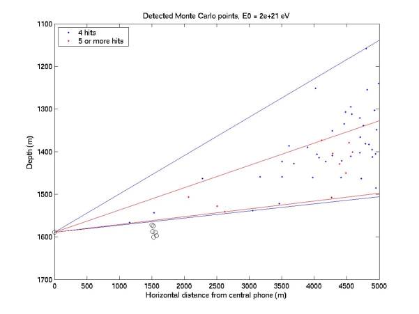
Figure 1

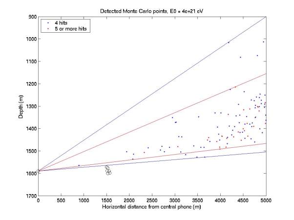
Figure 2

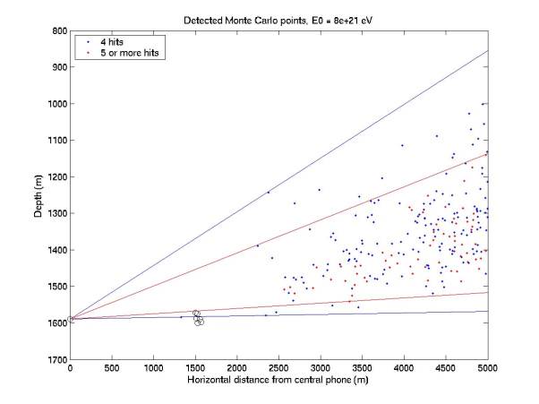
Figure 3

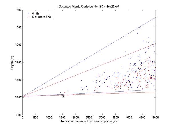
Figure 4

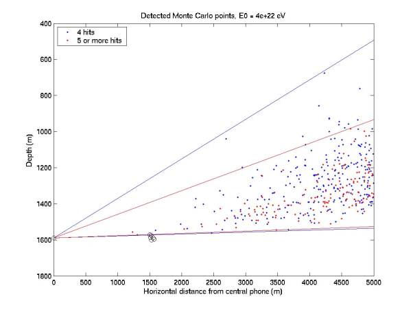
Figure 5

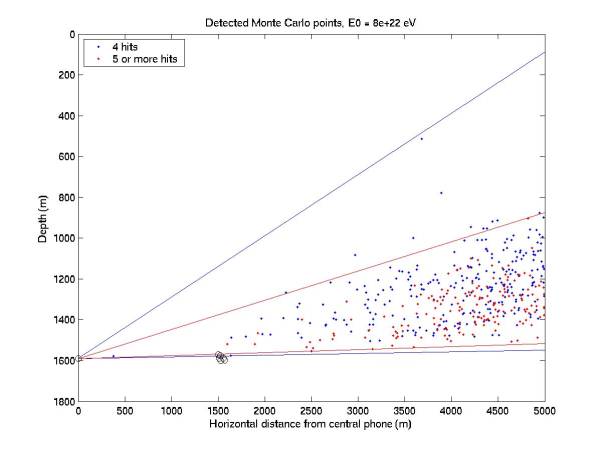
Figure 6

5/29/03

New waveform metric: crossings above threshold

plotThreshCrossings5Coin.m

I realized a simple waveform metric that could be quite powerful: counting the number of times the filtered waveform crosses above the online threshold. There are actually two quantities: first, how many samples are above threshold (depends on sampling frequency); second, how many times the waveform crosses above threshold (a measure of the number of periods in the signal; should be 1 for neutrinos).

I filtered each waveform and counted both samples above threshold and crossings (a crossing is a change from below threshold to above threshold). I calculated these parameters for all events in 5-fold coincidence. Figures 7 and 8 give histograms of these two parameters. There are some cases when both are zero. I don’t understand why this is.

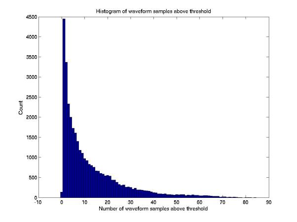
Figure 7

As shown in Figure 8, ~1/5 of the single-phone triggers (singles) in 5-fold coincidence have exactly 1 crossing above threshold.

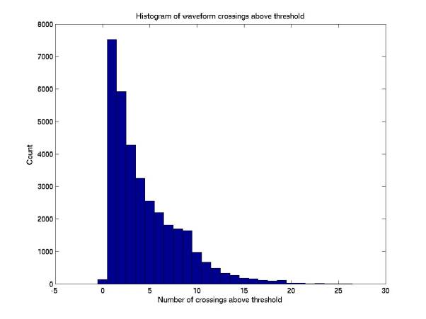
Figure 8

Figures 9-20 give pressure waveforms (upper panel) and filtered waveform (lower panel). A black line in the lower panel indicates the threshold. The color corresponds to the hydrophone that recorded the waveform. Note that, overall, the threshold choice looks quite good in these plots, despite the problems we’ve had setting an appropriate threshold. The title of each plot gives the number of crossings, the number of samples above threshold, the hour in which the event occurred (yyyy.mm.dd.hh), and the event number within that hour.

Pressure time series are given in Volts. To convert to Pascals, multiply by the gain, 14 Pa/V. Filtered time series are given in filtered Volts (arbitrary normalization).

Figure 9 shows an event that apparently never crossed above threshold. It’s a mystery why this event was recorded. There are O(100) of these.

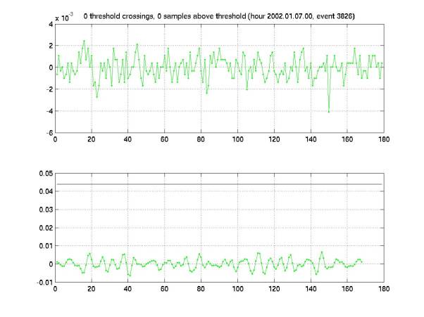
Figure 9

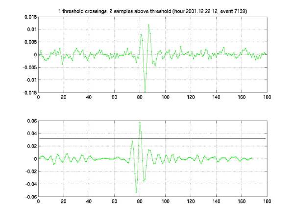
Figure 10

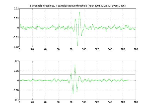
Figure 11

Diamonds account for many of the events with 6-16 threshold crossings.

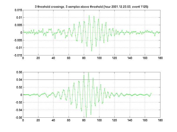
Figure 12

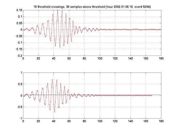
Figure 13

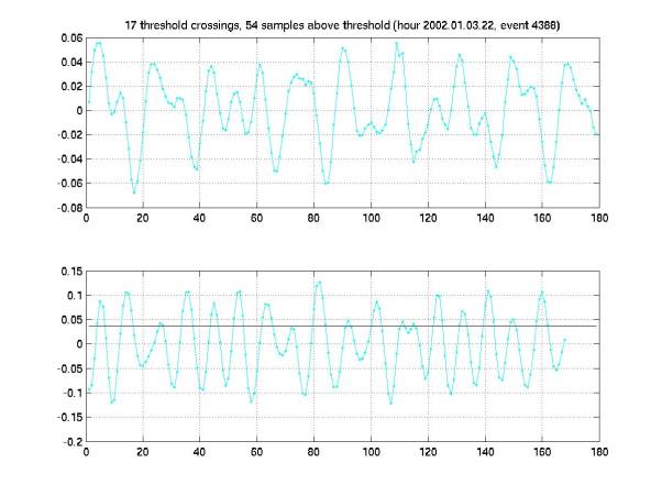
Figure 14

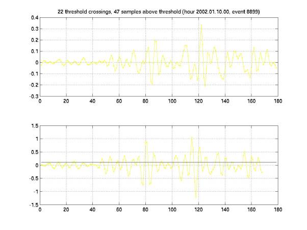
Figure 15

The event in Figure 16 hit the rails of the ADC.

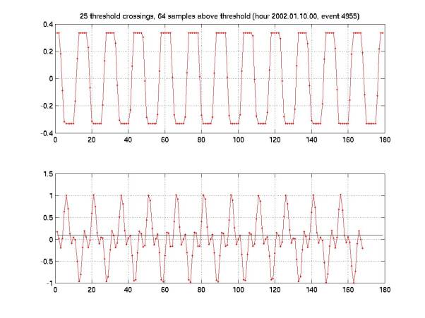
Figure 16

There are a bunch of events like Figure 17, a long damped sinusoid (perhaps part of a series of beats?).

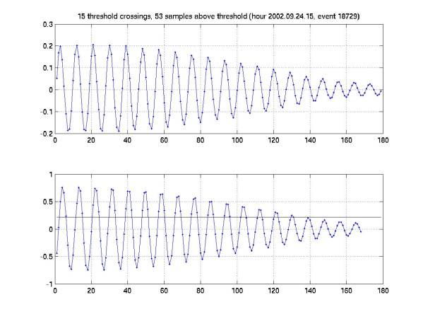
Figure 17

Figure 18 shows an event with beats with a much shorter beat frequency.

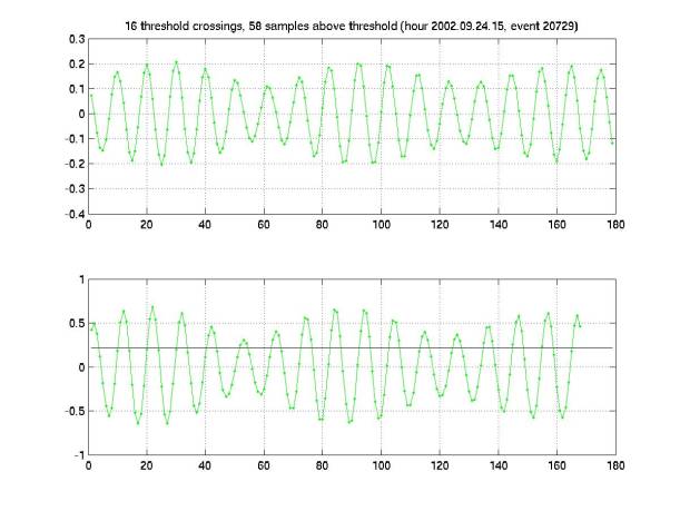
Figure 18

Figure 19 shows a sinusoid with constant amplitude (maybe part of a long beat).

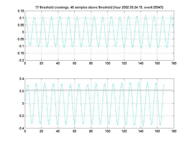
Figure 19

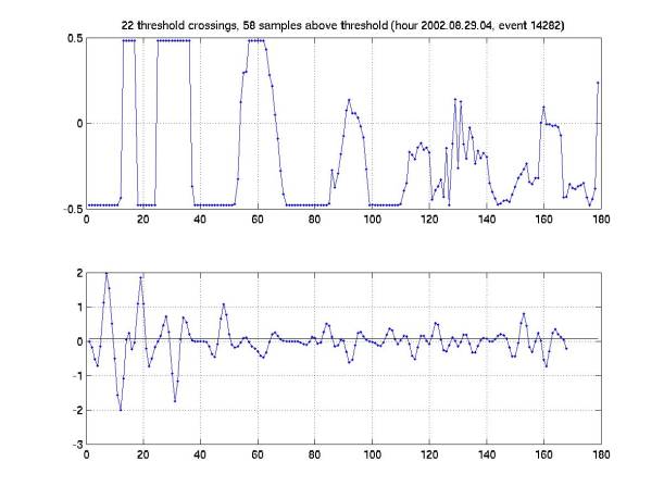
Figure 20

There are a couple potential problems with requiring only one threshold crossing. First, the threshold must not be set too low. If it is far too low, all events will have many crossings, (e. g. if the threshold is down in the Gaussian noise). Yet again, we need solid thresholding. Even if the threshold is awful and we have 10³ triggers in 60 s (with a target of 60 triggers), this is a small fraction of the number of triggers acquired if we trigger constantly. One trigger records 1 ms, so triggering continuously would be 6 x 10⁴ triggers, still 60 times more than our extreme example of 10³ triggers in a minute.

Unfortunately, because of the inadequate thresholding / event rate, we have periods in which we drop a buffer full of samples because we are swamped by data. This means we lose 17 s (if I remember right). So in the worst case there could be a couple of these in a minute so that we only record, for example, 10³ triggers when we should have had 10⁴ but missed some.

The second problem is the old problem of not knowing the effect of AUTEC’s bandpass filtering on neutrino waveforms (particularly the phase response). It could be that the filter transforms a bipolar neutrino waveform into a longer signal with multiple oscillations, and 2-3 crossings above threshold.