Log 22

Justin Vandenbroucke

justinv@hep.stanford.edu

Stanford University

This file contains log entries summarizing the results of various small subprojects of the AUTEC study. Each entry begins with a date, a title, and the names of any relevant programs (Labview .vi files or Matlab .m files – if an extension is not given, they are assumed to be .m files).

Note: Higher-resolution versions of the figures are available. If a log has URL dirname/logLL.html, Figure FF of the log should be at URL dirname/FF.jpg.

2/13/04

ADC range and saturation, and peak pressure distribution

pMaxDistribution.m

In an email 2/12/04, Naoko asked about the ADC settings. In SAUND-I Run II (also called Run B to avoid confustion with SAUND-II) data, the RMS pressure was of order 0.1 Pa. Typical loud events were 0.5 Pa; very loud events were 5 Pa. Figure 1 gives the distribution of peak pressures for all events from the first 1000 hours of Run B.

As shown in Figure 1, the ADC does saturate occasionally. However of the ~100 of these events I looked at, they were almost all diamond events, perhaps 1 or 2 multipolars. A handful of the diamonds looked like they extended way above 7 Pa, to ~20 Pa!

The ADC was set from –0.5 to +0.5 V, corresponding (with a gain of 14.1 Pa/V) to –7.06 to +7.06 Pa (before removing DC offset). The ADC is 12 bit, so there are 2^12 = 4096 values possible, with a step size of 1/4096 = 0.244 mV = 3.45 mPa. Looking at time series, the step size is indeed exactly 1/4096 V (not 1/4095).

If we know the gain of the new system, we can estimate what the ADC settings should be. They are restricted to a few discrete values, something like {…, ± 0.25 V, ± 0.5 V, ± 1 V, …}. I don’t see any reason to set the ADC range differently in different channels. The apparent variation in gain from phone to phone is less than a factor of 2, and our resolution is pretty good at 3.45 mPa (a thirtieth of the RMS).

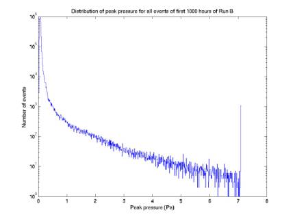
Figure 1

2/22/04

Effect of various transfer functions on mountain plot (Nikolai parameters)

plotTransfer.m

plotNP.m

Figures 2-5 give the simulated neutrino pulse after 4 possible transfer functions, A-D. The 4 are combinations of differentiation once and order-9 Butterworth bandpass filtering (7.5 – 55 kHz). Function (C) results in a signal somewhat similar to the tripolars, but with the two secondary ripples suppressed.

Figures 6-9 give contours enclosing MC neutrinos assuming each of the 4 transfer functions. There are 3 contours for each figure, enforcing a threshold of 0.00, 0.01, and 0.02.

Each contour encloses > 97% of the events above the relevant threshold, except for (C). The events from transfer function (C), differentiation extend to anomalously large frequencies and to negative characteristic number of cycles. I’m trying to figure out why this is.

The box shows the cut I have been using.

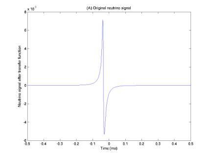
Figure 2

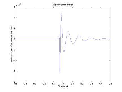
Figure 3

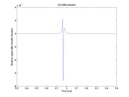
Figure 4

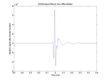
Figure 5

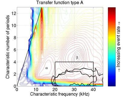
Figure 6

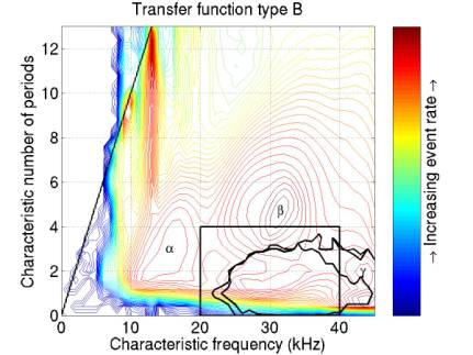
Figure 7

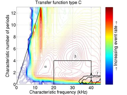
Figure 8

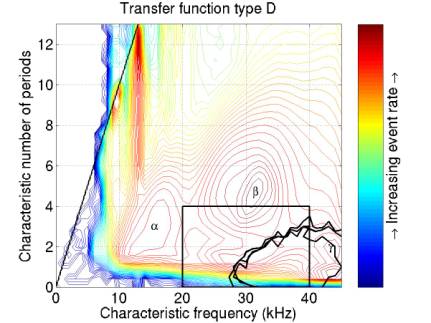
Figure 9

3/2/04

Added second derivative transfer function

plotTransfer.m

plotNP.m

Figures 10 and 11 give neutrino pulses after running through two new transfer functions, (E) twice differentiation, and (F) twice differentiation after bandpass filtering.

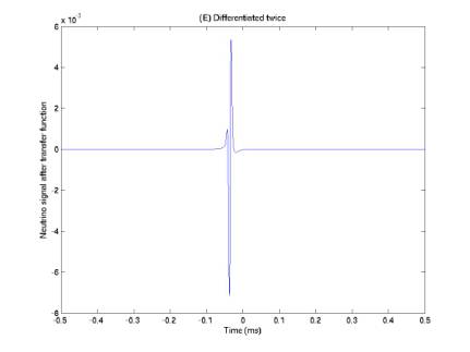
Figure 10

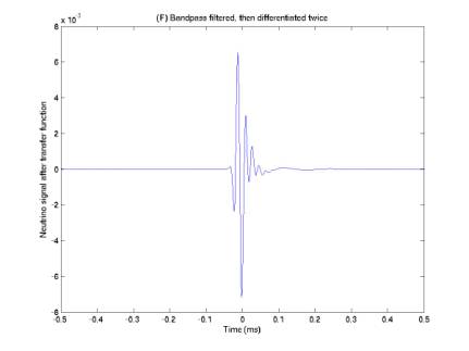
Figure 11

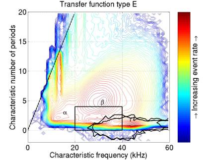
Figure 12

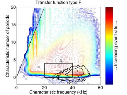
Figure 13

3/10/04

Efficiency of various transfer functions

plotFilterEff.m

Figure 14 gives neutrino efficiency vs. energy for the various transfer functions A through F. Each curves is determined from sets of neutrinos at particular energies. At each particular energies, a distribution of Monte Carlo events is built by filtering the neutrino signal and adding it to a noise sample chosen uniformly from the noise samples recorded every 10 minutes.

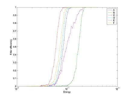
Figure 14

3/17/04

Light bulb energy calculation (again)

bulbEnergy.m

Figure 15 and Figure 16 are similar to figures given in Nikolai’s University of Hawaii talk. Figure 15 gives Nikolai’s simulated light bulb pulse, both unattenuated and attenuated with a smearing function. The energies (4*pi*r^2/rho/c) * integral(P^2 * dt) are 181 J and 152 J, respectively.

Figure 16 gives the energy spectrum on a log scale, for both the unattenuated and attenuated signals. Figure 17 gives the same spectrum S on a linear scale, and shows the total energy, (4*pi*r^2/rho/c)*integral(S * df), from 0 to 80 kHz (140 J) and from 7.5 to 55 kHz (62 J). So we expect to experimental signals of 62 J if the P*V -> acoustic energy conversion efficiency is 100%. According to the light bulb paper (PDF available on main SAUND page) however, this efficiency is only ~3-5 %. The actual signals we hear are 0.3 – 3 J, or conversion efficiency of 0.5-5%. The paper does note that efficiency decreases and becomes less predictable with greater depth, and is worst at failure depth, which is where we imploded the bulbs.

One problem: Nikolai’s theoretical signal is labeled as for a 3 cm diameter bulb, which would give P*V = 21 J, less than the radiated energy! Perhaps it’s actually for a 3 cm radius bulb (roughly what our bulbs were, standard “A19” sized household bulbs), which would give P*V = 166 J.

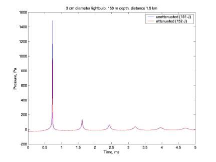
Figure 15

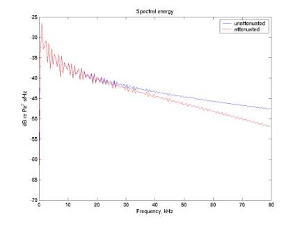
Figure 16

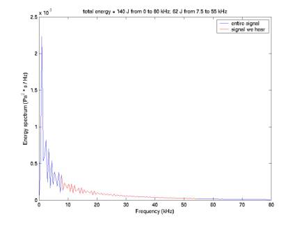
Figure 17

3/17/04

Logical ordering of cuts

plotNPCuts.m

Cuts have been applied somewhat haphazardly, in the order that we initially came up with them. This is not the most logical order or the best computationally. I reordered them so the quite noise conditions cut occurs first, followed by all waveform analysis (spike rejection, diamond rejection, correleated electronic noise rejection). I streamlined the implementation of these, so there are now ntuples calculated for all events – each event has associated with it 3 metrics for spike, diamond, and correlated noise rejection, and the threshold during the minute in which it was captured. So these 4 cuts can be tuned easily.

After these cuts have been applied, we can plot the Nikolai parameter (mountain) plot and reject events further based on effective frequency and effective number of periods.

Previously, several of these cuts occurred after looking for coincidence among events. I think doing all waveform analysis before the coincidence analysis will significantly reduce the number of coincidences (particularly from diamonds and spikes), and make this harder part of the analysis much easier.

Figure 18 gives a set of most (6 million of 8 million) events from quiet periods. It has been cleaned up from previous versions by increasing the resolution and removing all events from noisy periods (this removed a broad flat background). The band pass filter from 7.5 kHz to 55 kHz is evident.

Figure 19 gives only spike events (those with spike metric > 0.7).

Figure 20 gives only diamond events (those with diamond metric > 0.7).

Figure 21 gives all events from Figure 18 minus spikes and diamonds.

Diamonds and spikes are determined from independent metrics but are will-confined in Nikolai’s parameter space. It may be possible to remove these more aggressively while maintaining a high neutrino efficiency.

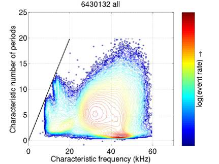
Figure 18

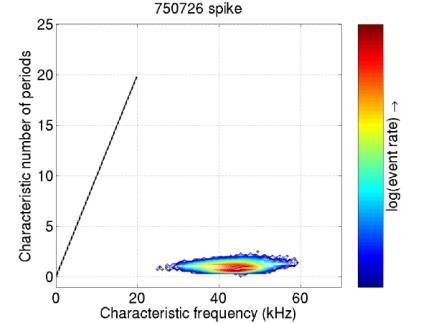
Figure 19

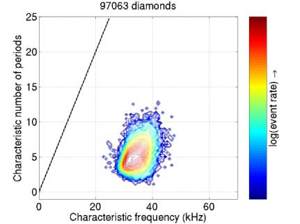
Figure 20

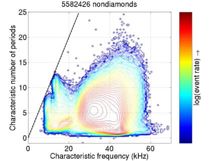
Figure 21

3/26/04

Various cut parameters calculated for Monte Carlo

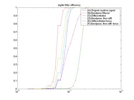
Figure 22

Figure 23

Figure 24

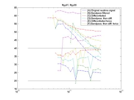
Figure 25

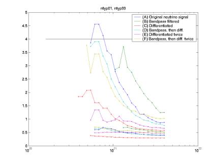
Figure 26

4/2/04

A good set of cuts

loadCutSet.m

applyCutSet.m

find5Concidences.m

plot5Coincidences.m

localize5Coincidences.m

plotLocalize5Coin.m

Table one shows a nice set of cuts. I’m still running on a handful of noisy time periods, but in the other time periods zero events survive all the cuts. For the events checked so far, note that no ntyp cut is necessary after all, which is good because it is a somewhat uncertain parameter due to uncertainty in the noise level (which is subtracted from the waveform). The ftyp cut is also soft.

1	any ntyp
2	ftyp > 25 kHz
3	trval > rethr (event trigger value > offline rehtreshold value)
4	rethr < 0.025 (low threshold / quiet conditions)
5	spike < 0.7
6	diamond < 0.7
7	event code = 0 or 1 (not 2) (don’t include small sample of events that didn’t pass online level 2 trigger)
8	0.5 deg < alpha < 20 deg (alpha is angle between event and horizontal as seen by central phone)
9	depth: z < 1550 m (the bottom 50 m are not included in our fiducial volume; reconstruction is awful)
10	Horizontal radial distance from central phone: 1 km < r < 4.5 km (also fiducial volume bounds)
11	Localization metric: m < 0.01 (a measure of localization convergence, corresponds to 100 m resolution - conservative)

Table 1