Log 25

Log 25

Justin Vandenbroucke

justinv@hep.stanford.edu

Stanford University

This file contains log entries summarizing the results of various small subprojects of SAUND. Each entry begins with a date, a title, and the names of any relevant programs (Labview .vi files or Matlab .m files – if an extension is not given, they are assumed to be .m files).

Note: Higher-resolution versions of the figures are available. If a log has URL dirname/logLL.html, Figure FF of the log should be at URL dirname/FF.jpg.

5/12/04

Rerunning with no effective frequency cut

plotNCoincidences(5)

with cutSetID = 2 (f_e > 25) or cutSetID = 5 (f_e > -1e10)

plotLocalize5Coin.m

I reran without the effective frequency cut. The number of events increased ~sixfold. Figure 1 gives number of events with the cut, Figure 2 without. Figures 3 and 4 give the resulting event maps. Actually these maps are incomplete – two hours of data had so many coincidence combinations it would take ~10 hours of running to complete them, and they have not been included.

Apparently the effective frequency cut is useful in beating down combinatorics.

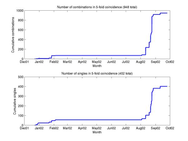
Figure 1

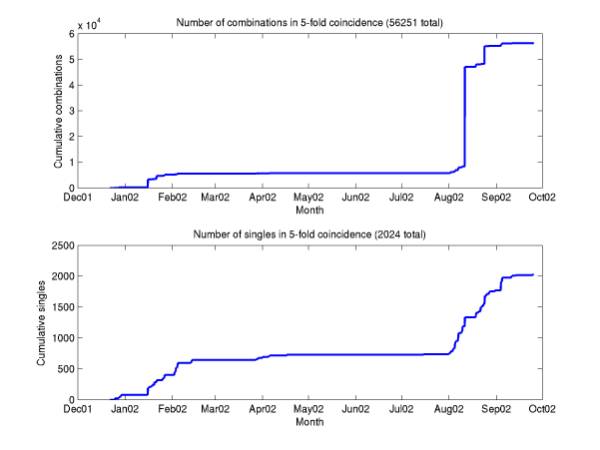
Figure 2

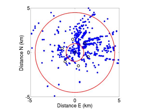
Figure 3

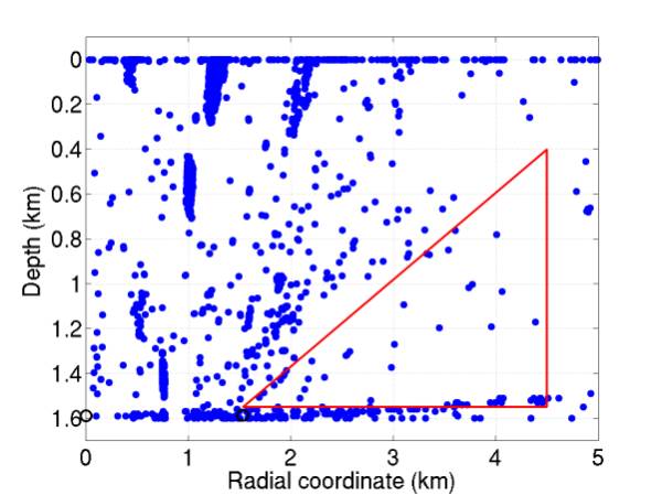
Figure 4

5/12/04

Neutrino cross sections, revisited

sigmaEstimate.m

plotSigmaEstimate.m

I looked at papers by Gandhi, Quigg et al again for extrapolations of neutrino-nucleon cross sections at UHE. I had been using a 1995 paper, hep-ph/9512364, but this was updated in a 1998 paper, PRD 58 093009. Both papers quote a power-law fit to energies from 10^16 to 10^21 eV. I extrapolate this as high as 10^32 eV (Figure 5) to find where the atmosphere becomes opaque, where the interaction length become 1000 cmwe. According to Figure 6, the atmosphere becomes opaque at ~10^32 eV. The new cross sections are lower than those in the previous paper by between 22% (10^21 eV) and 76% (10^32eV).

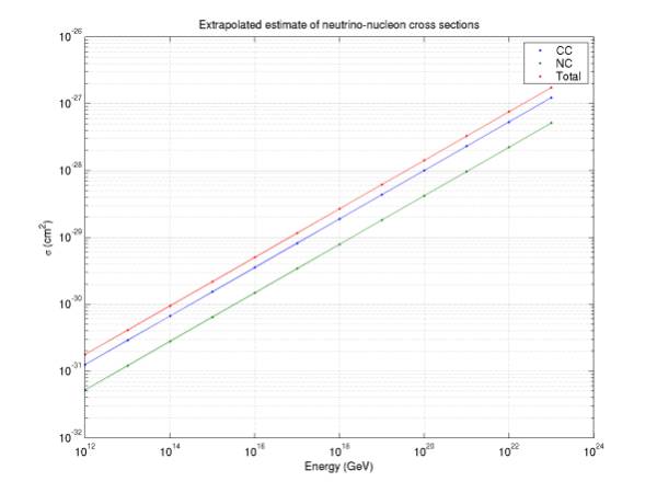
Figure 5

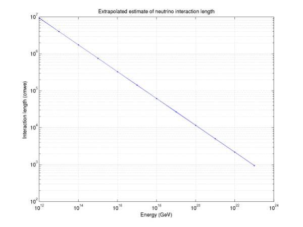
Figure 6

5/17/04

Radiation contours

plotDetectionVolumeRect.m (mode = small02, extraLarge)

The radiation contours in the current paper version only range from 5e20 to 3e21 eV, less than an order of magnitude, but we wish to calculate a limit over a range of ~4 orders of magnitude for comparison with FORTE. Figure 7 gives contours for 10^12 and 10^13 GeV. Figure 8 gives contours for 10^13 through 10^16 GeV. The bubbles at top and bottom are 10^17 GeV contours, hopefully they are glitches due to poor sampling and would be better resolved with an expanded mesh. This expanded mesh would be necessary to extend our flux limit to 10^17 GeV, currently it reaches 10^16.

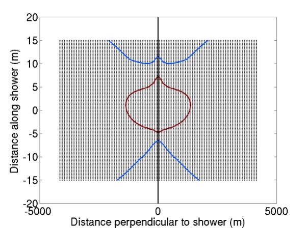
Figure 7

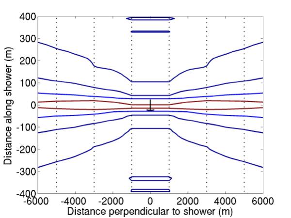
Figure 8

5/18/04

Final acceptance and exposure calculations

genMC.m

calcFinalAcceptance.m

calcExposure.m

Figure 9 gives “raw acceptance” (without multiplying by neutrino cross section), for various thresholds. Figure 10 gives “acceptance” (multiplied by N_A = 6.02e29 nucleons/m^3 and the total neutrino-nucleon cross section).

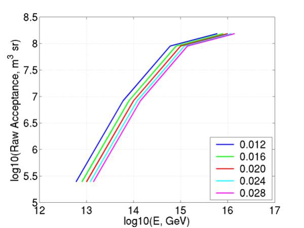
Figure 9

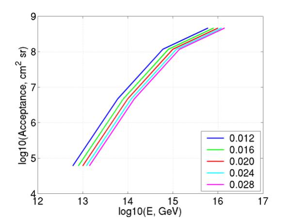
Figure 10

Figure 11 gives exposure, which is defined to be acceptance times livetime, at each threshold. Note that exposure increases with threshold (increasing livetime outweighs decreasing acceptance) until it reaches 0.028. This is how the “quiet conditions” cutoff (0.026) was chosen – above this threshold, the acceptance is too low to contribute significantly to exposure.

The black line gives the total exposure, summed over all thresholds.

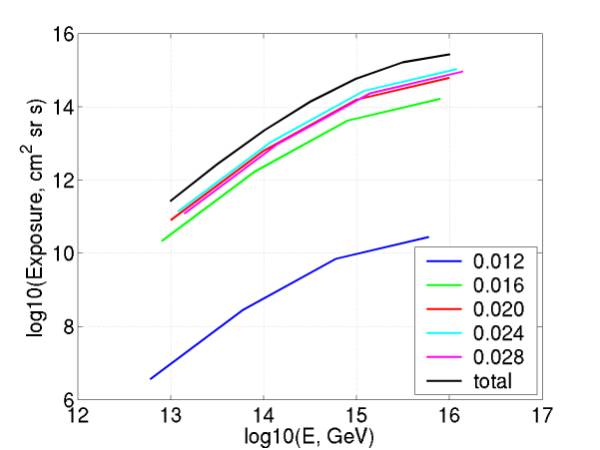
Figure 11

5/18/04

Final limit

finalLimit.m

Figure 12 gives our final neutrino flux limit (blue) compared to FORTE (red). At each energy, it is given (following the FORTE paper) by N times the energy divided by the exposure, where N is the Poisson upper limit at 90% CL given 0 events detected (N = 2.3).

If I’ve done it right, we’re 6 orders of magnitude behind FORTE. I’ve done some rough optimistic estimates that we could get into the regime of testing theories (z-bursts, td’s, grb’s and agn’s) with 1-km tubes sensitive along their entire length.

It looks like the best place such a detector could compete is about 10^12 GeV, where it could beat RICE and GLUE and test TD models. This particular detector would be 1 km strings spaced 500 m, spanning 10 km by 10 km.

The sensitivity of such a detector is roughly as follows: Assume we have the same energy threshold as currently (hopefully we can actually increase it), that is we can detect 10^21 eV neutrions at 1.5 km. Then assume the detector consists of 400 1.5 km vertical tubes spaced 500 m apart, spanning 10 km x 10 km. The effective volume is then V = (1 km)*(100 km^2) = 10^11 m^3. The maximum zenith detectable is roughly 45 degrees, corresponding to solid angle omega = 2*pi(*1-cos(theta_max)) = 2 sr (we assume a height of only 1 km, not 1.5 km, to allow this large solid angle). Assume livetime T = 1 yr = 3e7 s. Use NA = 6e29 nucleons/m^3, and assume sigma = 10^-31 cm^2 at 10^12 GeV. Then acceptance A = omega * V * NA * sigma, and exposure X = A * T, so our limit (GeV cm^-2 s^-1 sr^-1) is E/X = E / (omega * V * NA * sigma * T) = 2e-6. This is just above the TD predictions in the FORTE limit plot, and beats GLUE and RICE by 1-2 orders of magnitude. If we could gain an extra ~2 orders of magnitude somewhere, we could detect GZK neutrinos, the most solid theoretical source.

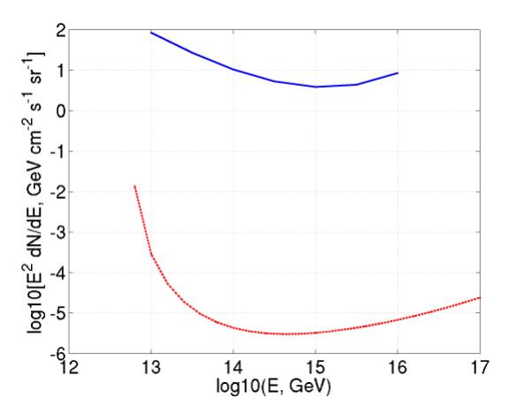
Figure 12

5/21/04

High-statistics MC for high-energy

goodMC.m

mcDistributions.m

We now have 2e5 MC events generated at each energy, of which ~ one in one thousand are detected. Distributions are given in Figures 13-18 for 10^16 GeV, for which 4e3 events were detected.

Figure 13 shows the most preferred zenith is not zero, or even ~1 degree (the tilt of the detector) but is ~10 degrees. Presumably this is because a couple km outside the array, the pancake needs to be tilted along the refracted ray back down towards the array.

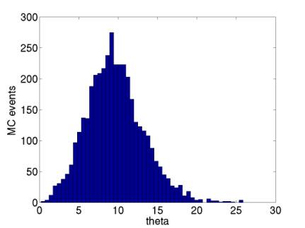
Figure 13

Figure 14 indicates there is some asymmetry in azimuth, presumably due to the sloping sea floor.

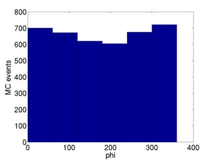
Figure 14

Figure 15 gives the distribution of radial coordinate of detected events.

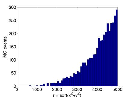
Figure 15

Figure 16 gives the side view of detected events. This is higher energy than was previously shown – this is why there are events above the triangle. Still it’s probably not worth extending the triangle to include the extra ~10% of events.

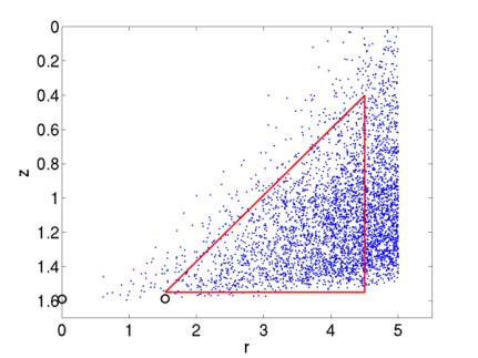
Figure 16

Figure 17 shows the top view of detected events.

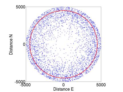
Figure 17

Figure 18 shows the correlation between phi (azimuth of incoming neutrino) and beta (if (x, y) is the location of the neutrino in rectangular coordinates, (r, beta) is the location in polar coordinates). I haven’t checked the exact direction of the correlation, but it’s a good cross-check that there is a correlation – this says that, outside the array, the pancake needs to point toward the array, not away from it.

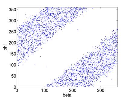
Figure 18

5/21/04

Log plot of detection contours

logContours.m

Figure 19 gives a log-log plot of the detection contours at 10^(11-16) GeV. It would be tedious but possible to extend the curves vertically and horizontally.

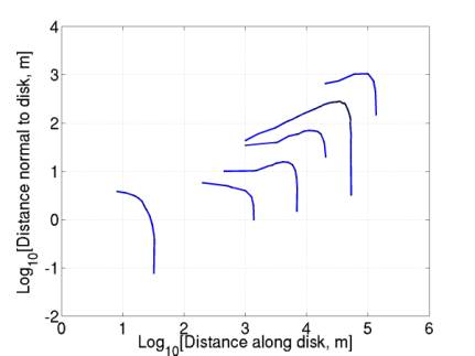
Figure 19

5/21/04

Pancake radius vs. neutrino energy

radiusVsEnergy.m

Figure 20 gives the pancake radius as a function of neutrino energy. Table 1 gives the same data. Note that the radius drops way down to 33 m at 10^11 GeV – presumably this is the far-field – near-field transition.

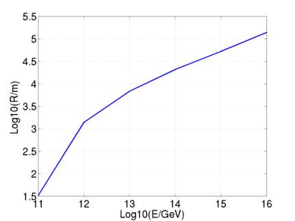
Figure 20

Log10(E/GeV)	R
11	33 m
12	1.4 km
13	6.9 km
14	21 km
15	53 km
16	140 km

Table 1

5/21/04

Limits and models

radiusVsEnergy.m

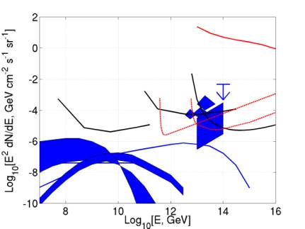
Figure 21