Results from Bottom Reflection Analysis, 7/30/2002

From December 22nd, 2002 to January 22nd, 2002, we have 32 days of almost continuously running period. We have 4,973,257 events recorded for about 2,764,800 seconds, which corresponds to an event rate of 1.7988 Hz (the target event rate is 1Hz). The entire data (from December 22nd, 2001 to June 14th 2002, with some breaks) set still has to be analyzed, and we have a total number of 6,311,460 seconds of data. Assuming the same event rate, we should have a total number of events of 11,353,054. The distribution of maximum amplitude (which is not necessarily the maximum amplitude of triggered channel) of events is shown in the following graph:

Among the 4,973,257 events, 884,375 (17.78%) have maximum amplitude higher than 0.5P. For bottom reflections, we only analyze events with maximum amplitude greater than 0.5P. Also, only about 10% of these events are recorded for 10ms in order to find bottom reflections (but actually we have about 30,000 events available for analysis from 12/22/2001 to 1/22/2002, which is only half the expected value, and it has not been well explained).

The next few paragraphs of this paper explain how we find a secondary signal following the original one and determine how similar it is to a bottom reflection signal following the primary signal. The essential tool developed is a fit function. Although the details about how the fit function works are not important to our analysis on bottom reflection in later paragraphs, understanding how it works will help the reader to realize the possible errors (hopefully only a few) in our analysis due to the limitations of the fit function.

Given an event, the fit function (1) tries to find the main component of the signal and treat it as the original signal, (2) tries to find a secondary signal that is similar in shape to the original signal and assigns it a value, called kai, to show the degree of likelihood (lower value of kai means that the secondary signal is more likely to be similar in shape to the primary signal), and (3) based on the current value of kai, performs necessary adjustments. All the three steps will be explained in details in the following paragraphs.

Up to now all the events we analyzed for bottom reflection consist of 1790 samples taken at a frequency of 179kHz (so the entire event is 10ms long). To find the main component of the signal, the fit function scans an event from the beginning to end, assigns each sample a number E (energy) that is equal to the sum of the square of the amplitudes of N samples leading that sample, N samples following that sample, and the sample itself (now this value is adjusted so that N = 10). Then, we find the sample with the largest value of E and treat it as the middle of the primary signal. The sample is named EX.

We also want to find the duration of the original signal since (1) we can only find bottom reflection after the original signal has ended – if the bottom reflection occurs before the original signal has ended it is hard to tell them apart, and (2) we do not want to misidentify part of the original signal as the bottom reflection. We require that the K (now K = 150, corresponds to 0.83ms) samples following the original signal to be relatively quiet in order for the original signal to be considered as ended. By quiet we mean the mean of the average energy of the K samples should be less than one percent of the maximum energy in the primary signal (that is, the energy at EX). There is some drawback in this method: if the bottom reflection signal is immediately following the original signal it is usually treated as part of the original signal and is rejected from further consideration (Later we will see that the distribution for the delay time between primary signal and bottom reflection signal has a lower limit of 1ms, which may partially be explained by this limitation of the fit function). Although in that case it is sometimes hard to tell whether we have a signal with two components or a signal with a reflection.

Note: the analysis done in the paper all uses the value K = 150, which imposes a lower limit of 1ms for delay time (finding delay time less than 1ms is technically impossible). As we can see later, sometimes it is desirable to get rid of the lower limit of 1ms for delay time. The analysis result we get by setting the value of K equal to zero is treated in another article titled “Epd.doc”.

Then we take M samples leading EX, M samples following EX, plus EX itself, to be the main component (now M is taken to be 15). We scan over the event from the sample where the original sample is considered finished, find the component of the event that is most similar in shape to the original signal. Specifically, we normalize the main component of the signal and the part of the signal we scan over by their energies (now the noise energy has not been taken into account), and take the sum of the square of the amplitude difference of the two, and name the sum d. Intuitively lower value of d means that the part of the event we scan over is more likely to be similar in shape to the primary signal. We find the smallest value of d for each event and call it the dev1 value for the event. The dev1 (which is also called kai) value, together with the position devx1 where it is obtained, is recorded for each event.

Sometimes it turns out that the component with the smallest value of d is clearly not the bottom reflection, even though it is the one that is most similar in shape to the original signal. The following graph shows such an example. The component of the event that has the lowest value of d starts at 1668, but clearly it is only a later part of the bottom reflection.

A few comments on how to read the event plot: for the event shown in the above plot (which will be standard in this paper), the graph on the top shows the primary signal (blue) and delayed signal (green) normalized by energy and plotted on top of each other, the graph on the bottom shows the entire event (blue) with the delayed signal (green) shown on their original scale.

In order to improve the situation, we perform the following adjustment: we find the mean value ME of d, take the difference between ME and dev1, and look for the earliest component of the signal devx1 that has a d value that is less than dev1 plus a fraction of the difference between dev1 and ME. If there is any, we name the starting position of that component devx2 and record the d value at that point as dev2, and we treat this component as the bottom reflection of the original signal. For the example given in the above paragraph, the starting point of bottom reflection signal is adjusted to 1109, which is clearly a much better choice. The following graph shows the event together with the deviation value computed for each sample superposed on it. Although the sample at 1668 has the lowest d value, the d value for the sample at 1109 is within a reasonable range and is earlier than the sample at 1668, so we take the sample at 1109 as the beginning of the bottom reflection signal. If dev2 exists for an event, we name it kai. Otherwise dev1 is named kai. Only a small fraction of all events need this adjustment, and it does not work well in some of the cases. But in general I regard it as a reasonable thing to do.

The fit function does not work perfectly. For one thing, there is a certain degree of arbitrariness in the assignment of the value such as M, N, and K. I can only say that the assignment now works reasonably well but there is no way that I can justify that they are the best choices. There are also some major assumption based on which the fit function works still need to be justified. We require that the bottom reflection signal to be similar in shape to the original one. If there is no bottom absorption, the reflectivity is frequency-independent, and before we reach the critical angle (about 60 degree), there will not be a phase change, so the shape of the pulse remains the same after reflection. After we reach the critical angle, the module of the reflectivity becomes one and there will be a phase shift. Now we hope that most of the interesting signals we get are simple sines and cosines.

Theoretically the kai value ranges from 0 to 2. Here is the distribution of the value of kai (*100) for all the events 12/22/2001 to 6/14/2002 analyzed.

A few comments on how to read plots in this paper: the x-axis and y-axis are very self-explanatory. The title indicates total number of events and the properties that events have to satisfy in order to be included in the graph. Dev is the kai value for the event, f is the frequency of the primary signal, l is the duration of the primary signal, r the Ed/Ep value (ration of energy of reflection signal to primary signal, or the square of the reflectivity), and p the periods of event. The p value is never used in this paper.

Frequency-duration and frequency-period analysis are very important for charactering events and separate them into different categories. Here are the two plots, which are done for the period for 12/22/2001 to 6/14/2002.

Frequency – duration plot:

Frequency-period plot:

There are two main groups of events, one below 23kHz, the other above 23kHz. For reason that will be shown later we now claim the events above 23kHz should actually be further divided into two subgroups, one from 23kHz to 29kHz, one from 29kHz to 36kHz.

We discovered that some events with low deviation values are actually very long sine waves. There are also events of other kind with low deviation values that are not good candidates for bottom reflection (however this is a more subtle matter to work with). These events usually have frequency below 23kHz. One example is shown below (sorry it is not standard plot):

Also, many events (although not the majority) in the range from 36kHz to 40kHz are electric spikes.

The following are two figures that show the typical events that fall into the frequency range 23kHz to 29kHz (first one), and 29kHz and 36kHz (second one). Note the small pulse very very close to the primary signal in the first graph – in this case it is unlikely that this is a bottom reflection signal, but even if it is, the fit function will be unable to pick it up since it is too close to the primary signal.

The distribution of deviation value for events whose frequencies are between 23kHz and 36kHz is as follows:

It is hard to assign a value of limit of kai below which the events are mostly likely to be bottom reflection. For example, events with kai approximately equal to 0.5 are pretty mixed – many are good candidates for bottom reflections but many others are not. Events with kai value less or equal to 0.25 are mostly good candidates for bottom reflection – keep in mind that the fit function is not perfect neither in assigning an exact value of kai nor in finding the delay time. Our following discussion will concentrate on the 2,172 events whose kai values are less or equal to 0.25, which accounts for about 10% of the events whose frequencies fall into the desired region from 23kHz to 36kHz.

If we reject all events whose kai value is greater than 0.25, the frequency-duration plot and frequency-period plots are shown in the following plot. Note: since now we only do analysis for events with kai value less than 0.25, the following analysis is done on a larger dataset, from 12/22/2001 to 6/14/2002. Now we can see why we further divide the events above 23kHz into two groups, one from 23kHz to 29kHz, one from 29kHz to 36kHz.

We can see that the frequency-duration plots, one for all events and the other for events with kai values less or equal to 0.25, are quite similar. Thus we can regard the fit program to be frequency-independent in general.

Also, from now on without explicit mentioning we assume that all the events we talk about are in the frequency range 23kHz and 36kHz. Also, lots of analysis later are done separately for two frequency ranges, one from 23kHz to 29kHz, one from 29kHz to 36kHz.

The following is the frequency-deviation plot. For this plot, the value of distribution above a particular frequency is normalized to the number of event at that particular frequency. It can be seen that in general the distribution of kai value is independent of frequency.

Probably the most important question concerning us here is to find the correct delay time of the bottom reflection signal. Following is the distribution of the delay time. Note that we have a physical limit of delay time of about 6ms due to the height (about 4.5m) of the hydrophone. It can be shown by simple geometry that the delay time dt is related to the angle of reflection alpha, the height of hydrophone h, and the speed of sound c by the formula: dt*c=2*h*sin(pi/2-alpha). This is an indication that the fit function picks up random signals sometimes. Hopefully later we will show some of the special properties of those random events so that we can start finding ways to reject them.

Here is the distribution of the duration of signal.

A lower bound of the delay time at about 1ms exists. Keep in mind that there is a limit where the reflection angle alpha approaches 90 degree and delay time approaches 0. In that case, the original signal and the reflected signal merges. Later we show that the duration of the original signal, as assigned by the fit functions, centers around 0.5ms. Also as we have shown, the fit function simply cannot extract the reflected signal from the original one. The 1ms lower bound may also be the result of the limitation of the fit function due to the way in which the fit function is implemented as explained at the beginning of this paper.

Also the speed of sound in water is a function of depth. Thus depending on the origin different signals will be bent in different ways as they propagate, and this may result in a preferred direction of propagation and thus a preferred direction of reflection angle.

Energy analysis.

As we are looking for bottom reflection signals, we at the same time determine the energy of the primary signal and bottom reflection signal. Here we show the analysis done that is related to the energy of the initial/primary signal (Ep) and energy of the reflected/delayed/secondary signal (Ed). Note that here Ed/Ep is equivalent to the square of the reflectivity.

Because fit function always picks the component with the largest energy as the primary signal, it is not surprising that Ed/Ep is always less than 1.

Note that on this plot, events general fall into two categories – one category with Ed/Ep less than 0.05, the other with Ed/Ep greater than 0.05.

For events with delay time longer than 6ms (which means that they cannot be bottom reflection candidates, but rather they are random signals following the primary signal), we can see that they mostly belong to the category where Ed/Ep > 0.05. In other words, the energy difference between the delayed signal and the primary signal becomes smaller. This makes sense – since the secondary signals are random there should not be a significant difference between energies of the secondary signals and the primary signals.

	23kHz – 29kHz
	Ed/Ep < 0.05	Ed/Ep > 0.05
d < 6ms	2327 (89.88%)	209 (8.07%)
d > 6ms	44 (1.70%)	98 (2.79%)

	29kHz – 36kHz
	Ed/Ep < 0.05	Ed/Ep > 0.05
d < 6ms	5337 (87.97%)	395 (6.51%)
d > 6ms	142 (2.34%)	193 (3.18%)

Another example shows that the events with Ed/Ep > 0.05 are more likely to be random signals comes from the distribution of delay time. For bottom reflection signals, the delay time should be within 6ms of the original signal. But for random signals there is no such restriction. The plot for events with Ed/Ep > 0.05 shows little respect to the limit of 6ms.

The following plot intends to show the possible dependence of Ed/Ep on frequency. It appears that the relative distribution of reflectivity for events whose frequencies are from 29khz to 36kHz is approximately the same, with a concentration at Ed/Ep value below 0.025.

Very naturally the reflectivity should depend on grazing angle. The following graph shows this feature. The red line and black line correspond to one percent of the square of the real part of reflectivity and imaginary part of reflectivity, respectively. The reflectivity is calculated such that no absorption is assumed, sound speed in seawater to be 1,513m/s, sound speed in sea-floor is 1,750m/s, the density of sea-floor to be 1.8 times the density of seawater. The critical angle in this case is 59.83 degree. Note that the x-axis has a certain degree of arbitrariness. Remember that the formula relating the reflection angle and delay time is dt*c=2*h*sin(pi/2-alpha), but the parameters c and h (especially h) are exact, so it is very possible that the blue dots on the plot will be shifted horizontally, although to which direction I do not know.

It seems that there is certain correspondence between Ed/Ep and the real part of reflectivity, especially for angle beyond critical angle. But now we do not know how to take into account the phase shift (the imaginary part of reflectivity). Also it seems that bottom absorption is really high (remember the red line is one percent of the square of the reflectivity).

Variation of number of events during different time of day

The events with frequencies from 29kHz to 36kHz are not random signals. Their number of occurrences depends on the time of the day, especially for the group with frequency from 23kHz to 29kHz.

Here is the distribution of time interval between such two events. Unfortunately this plot is not as meaning as one can expect since the events listed here only account for 10% of the total events recorded.

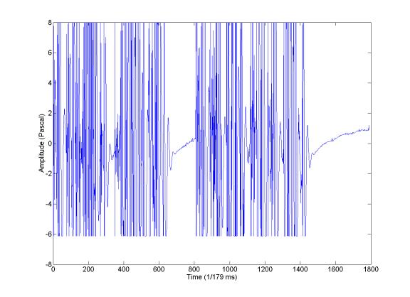
A kind of very special signal that is only recorded on channel one

There is a very interesting (for several reasons) kind of event. It happens to look like the neutrino event predicted by Nikolai. Many of these events have really high amplitude (over 7 Pascal), and many come in close succession. But very strange it only happens on channel one as I have observed so far, so it is unlikely that it is acoustic event.

Here are some of the examples of such events:

Also it seems that this kind of signal have a DC drift sometimes (which gives a really high kai value).