Note: all the MatLab programs that I have used are in C:\AUTEC_analysis\m_files directory. Most, but not all of these programs end with a letter y. Several are only slightly modified from Justin’s program, such as ReadEventRecordy.m.

Some useful programs

Constructdirsy.m: construct the name for directory in AUTEC_analysis folder, generic for Hep 26 and Hep 14. I believe that Justin has programmed something similar, but I have kept using this program.

Validdayy.m: it generates an array d and save it in the file validday.mat in mat files\validdayy directory. The element of array is such that d(year-2000, month, day) = n, where the value of n has the following meaning:

0: no data for that day exists.

1: the data for that day exists, and has file format 1.

2: the data for that day exists, and has file format 2.

3: the data for that day exists, and has file format 3.

Note: d(1,…,…) actually refers to year 2001, similarly, d(2,…,…) refers to year 2002.

You should run validdayy.m to update the content of d whenever new data is added to or the old data is deleted from the computer. The data stored in n only reflects the data actually stored on Hep26. It does not take into account the data stored at other places.

The specific command to load d in a Matlab program is as follow:

f = fullfile(constructdirsy('mat files'),'validdayy','validday.mat');

load(f)

EventCount.m: this program is very similar to Justin’s eventlist, but with slightly more outputs. It inputs a time vector to its subprogram EventCountSub.m, which outputs an 2-D array n2. EventCount.m then combines the minutely data in an hour to a 2-D array n and store it in the file EventCountIyear.month.day.hour.mat (note the letter I!) in C:\AUTEC_analysis\mat files\EventCountI.

Each row of n corresponds to a single event. Each one of 8 columns of n corresponds to a property of the event. The data format in a single row is as follows (number in parenthesis is the column number):: [le(1) dn(2) t0(3) identifier(4) trchan(5) tramp(6) mchan(7) mamp(8)], where le(1) is the local event number, dn(2) the date number, t0(3) the time stamp, identifier(4) is 0 if the event has 179 samples, 1 if 1790 samples, trchan(5) the triggered channel, trchan(5) the maximum amplitude in triggered channel, mthan(7) the channel with maximum amplitude, mamp(8) the maximum amplitude in maximum channel.

EvnetCountSub.m as implemented now reads the time series of each event. So we need to be really careful which event reading program we are using, and whether we have performed scale and DC correction. Now all the files in the folder EventCountI are generated without DC removal and scale correction.

There are several programs that use the data file generated by eventcount.m. They are:

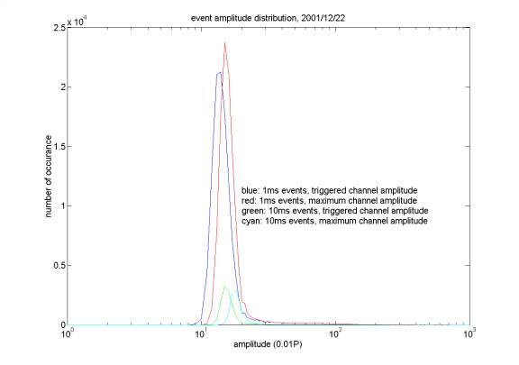
Ecampy.m (event count amplitude): plots the histogram for triggered amplitude, maximum channel amplitude for 1ms and 10 ms events. The range of date used can be manipulated in the program. Here is an example for events on 2001/12/22:

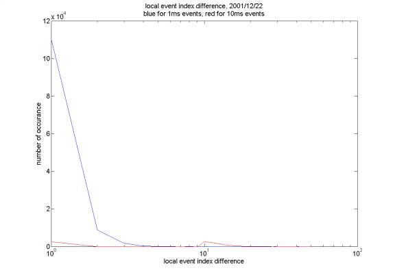
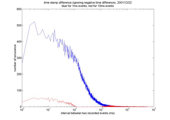
Ecdley (event count difference le): this program generates two plots, the first one is the local event index difference separately for 1ms events and 10ms events (of course the difference is always one in a single minute), the second one is the time stamp difference between 1ms events and 10ms events.

Note that there are 10ms events with time stamp difference less than 10ms, which signals an error in the trigger program.

DataCount.m: it generates an array c and save it in the file datacount.mat in mat files\datacount directory. The element of array is such that c(year-2000, month, day hour) = n, where n is the number of events for the given hour (from 1 to 24).

You should run datacount.m to update the content of c whenever new data is added to or the old data is deleted from the computer. The data stored in c only reflects the data actually stored on Hep26. It does not take into account the data stored at other places.

The specific command to load d in a Matlab program is as follow:

f = fullfile(constructdirsy('mat files'),'datacount','datacount.mat');

load(f)

Bottom Reflection

Br7y.m is the program that generates the files with necessary information for bottom reflection analysis (there are a series of bottom reflection analysis programs, from br1y.m to br7y.m, which reflects the evolution history of bottom reflection analysis). Br7y.m is associated with a subprogram brmin7y.m, which does the analysis for a given time vector. Br7y gives time vector (dv) to brmin7y.m, and take output (an array ts3) from it, and combine the data from each minute in an hour, and save the hourly data – an array tst – to a file. The file is in the directory C:\AUTEC_analysis\mat files\Bottom Reflection\br7y(0.5P), or C:\AUTEC_analysis\mat files\Bottom Reflection\br7ky(0.5P) – 0.5P reflects the fact that the analysis was done for events with maximum amplitude greater than 0.5P.

The format of the file name is br7yyear.month.day.hour.mat or br7kyyear.month.day.hour.mat. The difference between br7y and br7ky files is that the analysis stored in br7y files was done with the condition that k = 150 (which basically results in a lower limit of delay time of about 1ms), while for br7ky files the value of k is set to zero (no lower limit of delay time). The meaning of the value of k is explained in Bottom Reflection5.doc.

The 2-D array tst stored in these files are as follow: each row corresponds to a single event analyzed. There are 27 columns, each column corresponds to a data value.

For each row (which corresponds to a single event) the data is in the following format (number in parenthesis is the column number): [dv(1-6), le(7), t0(8), trchan(9), ts2norm(10), devx(11), dev(12), devnorm(13), tt(14), ft(15), nt(16), jc(17), ev(18), ze(19), re(20), lr(21), l1(22), s1(23), ye(24), devx1(25), dev1(26), devnorm1(27)].

More specifically, dv(1-6) is the time vector in the usual format (year month day hour minute second), le(7) is the local event index within the minute given by the time vector, t0(8) is the time stamp, trchan (9) the triggered channel, ts2norm(10) the energy density of the primary signal, devx(11) is starting point of the bottom reflection, dev(12) the kai value assigned to the event, devnorm(13) the energy density of bottom reflection, tt(14) the length of the primary signal, ft(15) the typical frequency of the primary signal as calculated from Nikolai’s program, nt(16) the periods (number of cycles) of the signal, jc(17) the correlation probability between different channels as calculated by Nokolai’s program, ev(18) the event category, ze(19) the exact starting point of the primary signal, re(20) the ending point of the signal (also where we start searching for bottom reflection if k = 0), lr(21) is basically re-ze+1, l1(22) = 15, s1(2) the starting point of the component of the primary signal (now set to 31 samples) that we take to compare to all the other part of the signal, ye(24) is where we start searching for bottom reflection if k = 150. devx1, dev1, devnorm1 can be ignored for now (those are the result we get before we make the adjustment as mentioned in Bottom Reflection5.doc).

Important hourly br7yyear.month.day.hour.mat combine program: since we usually work on the entire dataset rather than data file generated for each hour, we have several programs that combine hourly data file into a single larger data file. This is done in different steps using various br%sy files, where s can be c, cc, ccc, or cccc. The details about how these programs work can (hopefully) be easily figured out by reading the code, but it is better to just use the larger data file generated by them. The larger data files have the format as (although there are files with other format, they can be ignored for now):

Br7%sy(0.5P)tst%d(%.2f).mat,

where s = “” (indicates that it is generated by br7y.m) or s = “k” (indicates that it is generated by br7ky.m). d = 2 (indicates that events are in chorological order) or d = 3 (events sorted in ascending order by kai value). f indicates that all the events considered in that file have upper kai limit equal to f.

Various Bottom Reflection Analysis Programs: there are many programs that generate plots as the results for bottom reflection analysis. These programs usually start with letter br7 (some starts with br) followed by various combination of strings listed below:

Ep: Energy density of primary signal.

Ed: Energy density of bottom reflection

Epd: ratio of energy density of primary signal to energy density of bottom reflection

d: delay time

l: duration of primary signal

p: periods of primary signal

f: frequency of primary signal

X: kai value

angle: reflection angle as calculated by delay time

and followed by a letter ‘y’ at the end.

So the analysis program usually have the format (1) br7y%sy.m or (2) br7y%s1%s2y.m, where %s is one of the strings listed above. If the program is in format (1), it usually means the program generates a histogram for property s. If the program is in format (2), it usually means that the program generates scatter plot for property s1 verses s2 (or s2 verses s1, the order is not strict).

(Sometimes the program generates contour plot for property s1 verses s2, and it may be indicated by the letter ‘c’ at the end.)

I am sorry how these lettered are arranged is sometimes random.

Event Selection Program: for most cases we are interested in doing analysis for certain frequency, period, and duration range, i.e. restrict our attention to some island on frequency-duration/period plot (of course the exception is that when we want to do make contour plot for frequency-duration, frequency-period for all frequency, duration, period range). Thus, there is an event selection program to choose event satisfying some conditions. The program is now named br7SelectEvty.m, which is used in the following format:

tst3= br7SelectEvty(tst3, devl, devh, fmin, fmax, lmin, lmax, rmin, rmax, pmin, pmax);

The meanings of the parameters are explained as follows:

devl: the lower limit of the kai value for the desired events

devh: the higher limit of the kai value for the desired events

fmin: the lower limit of the frequency range for the desired events

fmax: the higher limit of the frequency range for the desired events

lmin: the lower limit of the delay time for the desired events

lmax: the higher limit of the delay time for the desired events

rmin: the lower limit of Initial Energy/Delayed Energy ratio for the desired events

rmax: the higher limit of Initial Energy/Delayed Energy ratio for the desired events

pmin: the lower limit of the periods range for the desired events

pmax: the higher limit of the periods range for the desired events

The implementation of br7SelectEvty is easily understood and should be easily updated if additional selection options are needed.