In “Bottom Reflection5.doc” we mentioned that by setting the value of K equal to zero we remove the lower limit of delay time of 1ms. In this article we concentrate our analysis result we get by setting the value of K equal to zero.

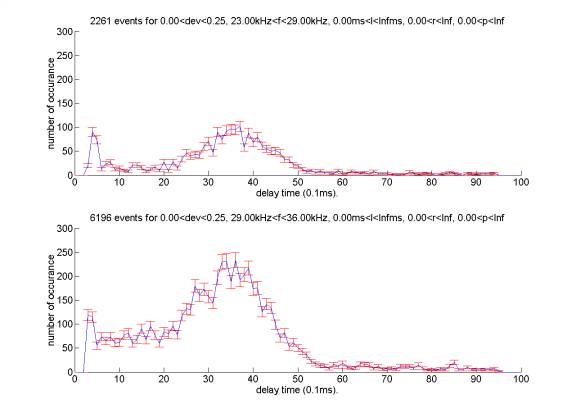
Here is the delay time distribution:

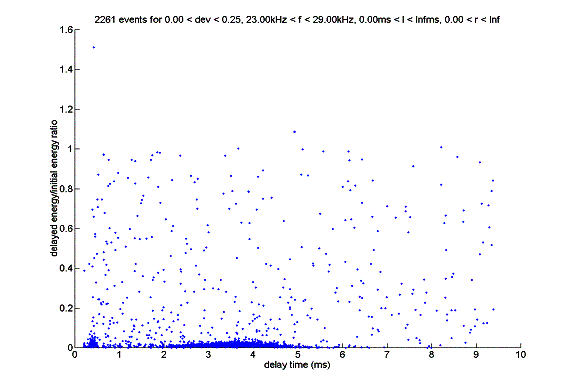
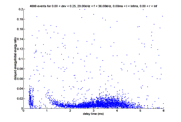
The reflectivity – delay time (grazing angle) plot for frequency range 29kHz to 36kHz is as follows:

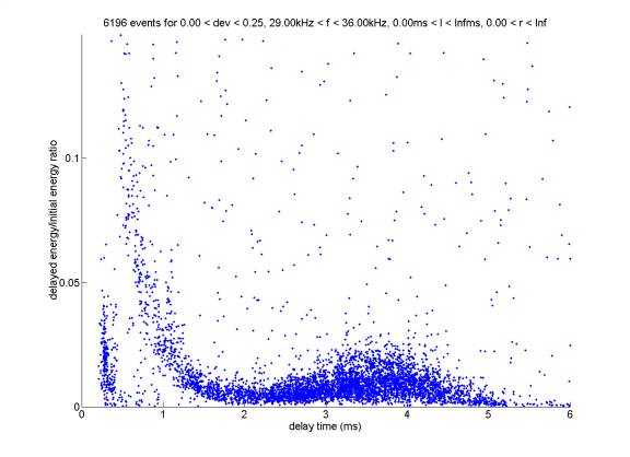
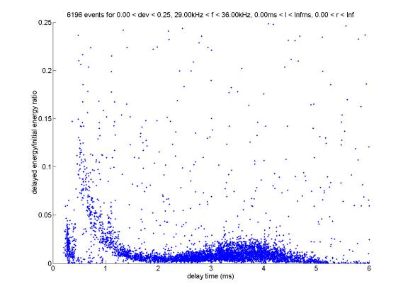
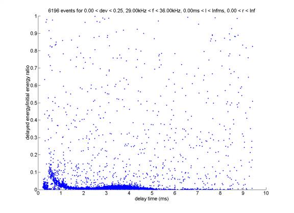
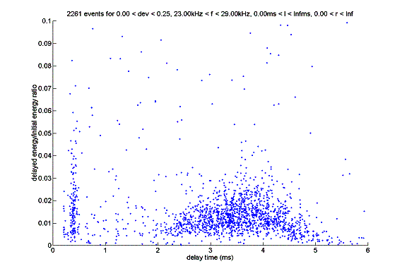
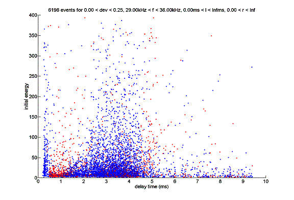
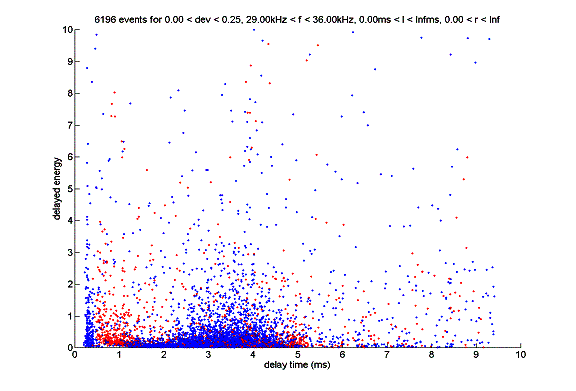
(The above three plots only differ in scale)

Event needed for the paragraph below:

One interesting change after we set the value of K to zero is that we can see an increase in reflectivity for events in the frequency range 29kHz to 36kHz, if their delay time is relatively low (later we will see what could have caused this phenomena). These events are mostly included in the green box in the above plot. This feature was not seem before when we set K equal to 150, since doing do basically eliminate the possibility of assigning a low delay time for any event. Some of the examples of the events in the green box are shown in the file “Epd1.doc”.

Plot for the paragraph below:

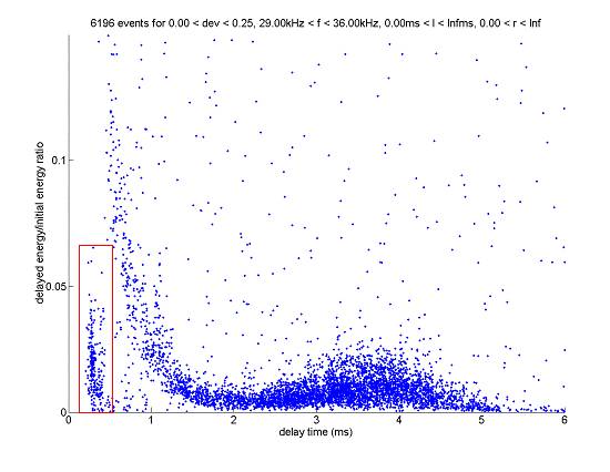
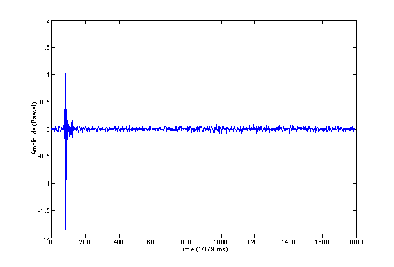
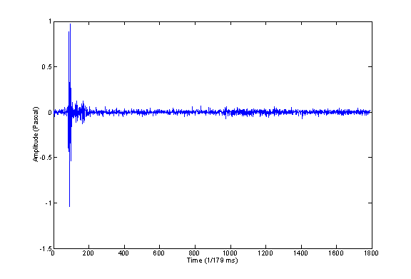
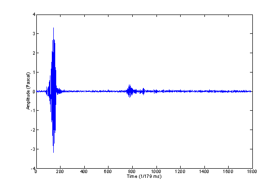
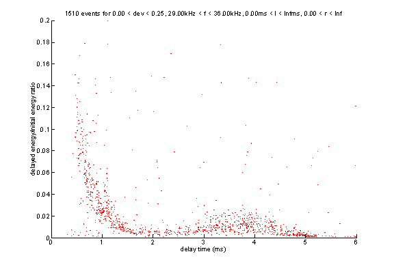
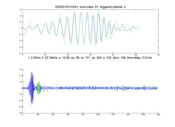
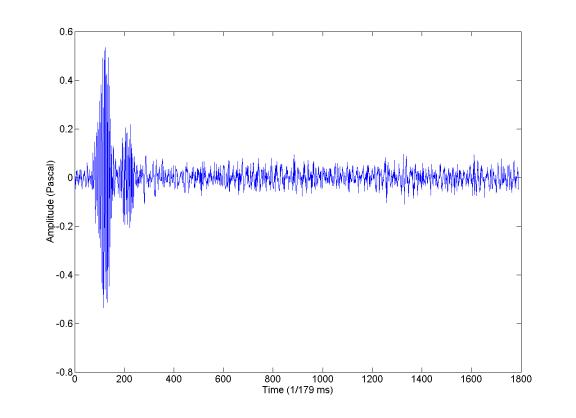
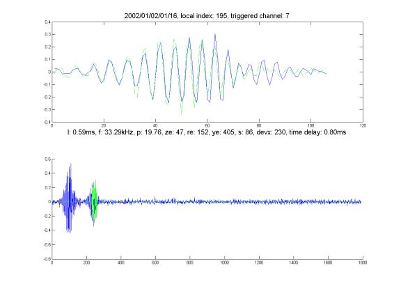
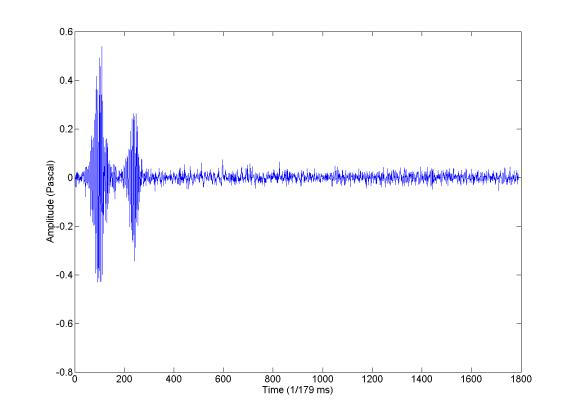
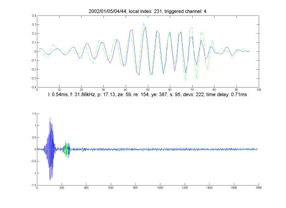
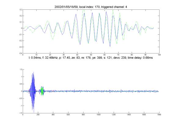
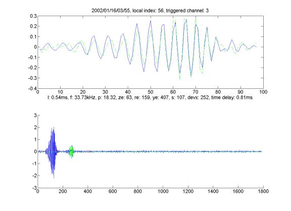
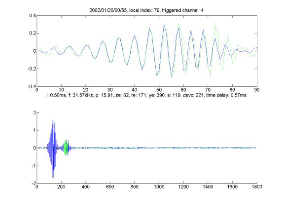
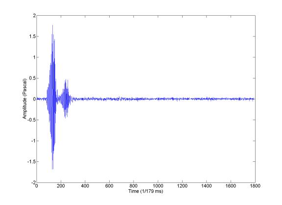
Another noticeable feature is that a cluster centered at approximately 0.28ms and Ep/Ed value less than 0.1 (the events in the red box). Those events, with four typical examples shown below, basically have a double structure – a primary signal immediately followed by a much smaller signal. But usually recognizable bottom reflections occur much later, which means that those events are usually assigned incorrect delay times. The secondary signals picked up by the fit function are not actually bottom reflections. Some of the examples in the red box are shown in the file “Epd2.doc”.

Actually much more analysis was done on the events in the red box to show that they are not bottom reflections. Lots of examples are included “Bottom Reflection7.doc”. These events are further grouped into several categories mostly according to their shapes and these different categories are saved in the file “BR6mslimit.doc” (bottom reflection occur at about 6ms limit), “BR6BackDiamond.doc” (bottom reflection with some distinct shape), “BRFunny.doc” (funny bottom reflections), “BRPeakFollowedByTail.doc” (bottom reflections are a peak followed by a tail), “BRWithoutObviousBR.doc” (without obvious bottom reflections), “BROther.doc” (other bottom reflection). It must be interesting to find out why bottom reflections have different features (shapes), but I think it will be too complicated.

Reflectivity – grazing angle for frequency range 23kHz to 29kHz.

We can see that the cluster of events with delay time centered at 0.28ms and Ep/Ed value less than 0.1 also exists for this frequency range (the events in the red box for frequency range 29kHz to 36kHz). But the increase in reflectivity (the events in the green box for frequency range 29kHz to 36kHz) are absent in the above plot. This may signify that events in two different ranges are from at least two different sound sources.

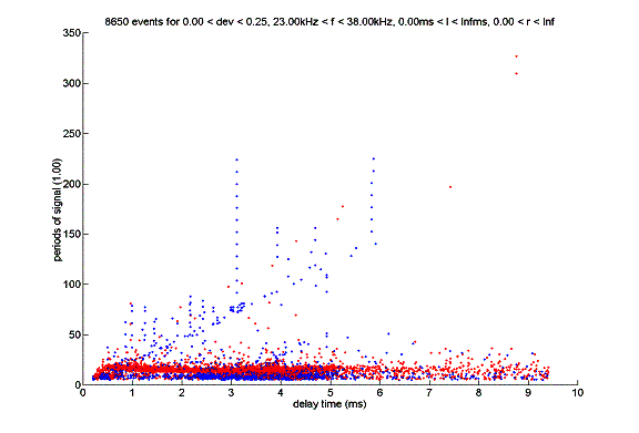
The increase in reflectivity for events with delay time less than 2ms motivates us to do periods – delay time, duration – delay time, frequency – delay time analysis.

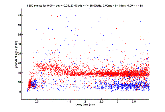
Here is the periods – delay time plot (blue for events from 23kHz to 29kHz, red for events from 29kHz to 36kHz):

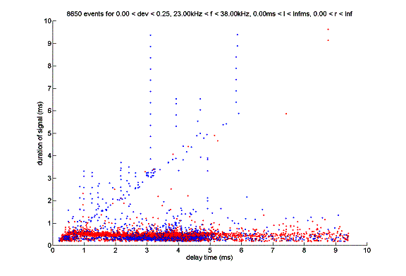
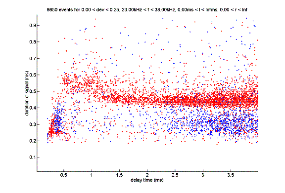
Here is duration – delay time plot:

Plot for the next paragraph:

We can see that there seem to be a group of events with slightly longer duration time whose period is generally greater than 15.8, in a frequency range from 29kHz to 36kHz (the events in the black box in the above plot). If we plot reflectivity – delay time for these events separately, we get the following picture:

On the other hand, the reflectivity – delay time for events with periods less than 15.8 within the frequency range of 29kHz to 36kHz, is as follow:

We can see that events whose periods are greater than 15.8 nicely account for almost all the events that cause the increase of reflectivity the events with shorter delay time. Thus we conclude that there might be some reason that these events are actually from a different sound source that provides more detailed information about reflectivity – grazing angle relationship.

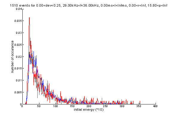
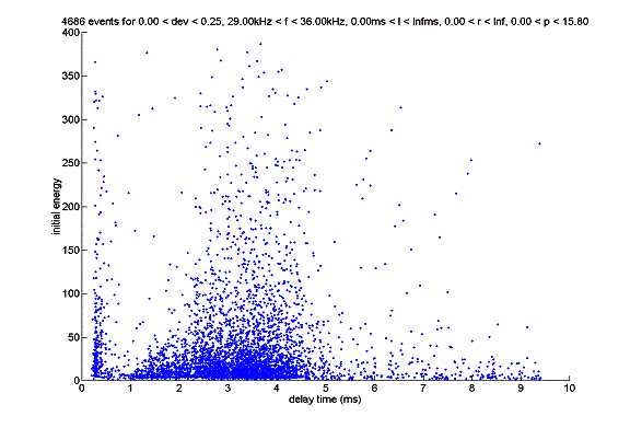
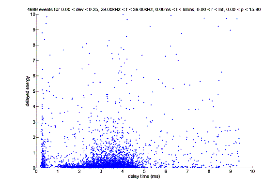
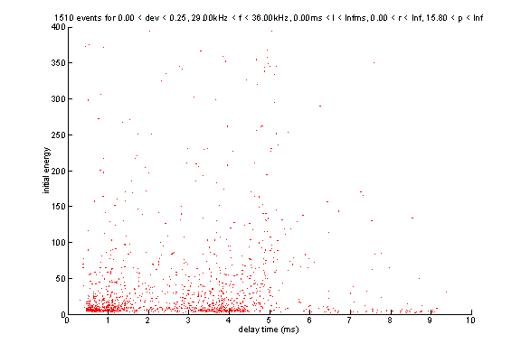
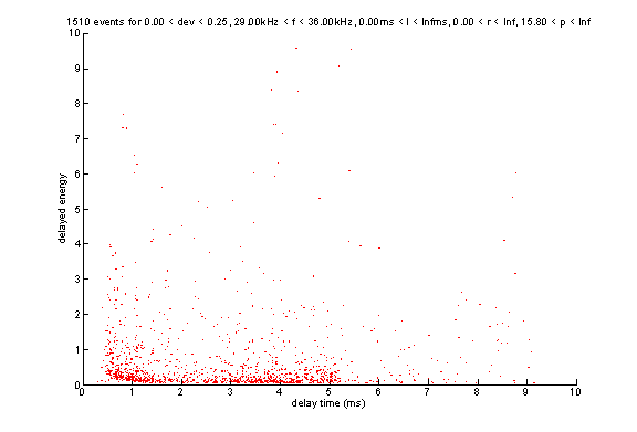
It is also interesting that initial energy and delayed energy distribution themselves are dependent on grazing angle. In the plots below red points correspond to events with periods higher than 15.8, blue points below 15.8.

Initial Energy fractional distribution (red for periods greater than 15.8, blue for less).

Initial energy – delay time plot for events whose periods are less than 15.8:

Delay time – initial energy plot for events whose periods are greater than 15.8. Note the absence of cluster for delay time less than 2ms for these events.

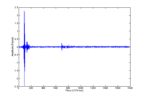
Some examples for events with periods greater than 13.8 and low delay time, Ep/Ed > 0.02. We believe that these are the bottom reflection events.

Events with relatively high amplitude but no obvious bottom reflection happening much later – it may indicates that the secondary signal may be the bottom reflection.

End.